Knowing how to calculate the cumulative count of distinct values can be helpful in many ways. For example, you can use it to track how many unique customers have made a purchase over time or count how many different products have been sold cumulatively.

In Google Sheets, you can use the SCAN function to get the cumulative count of distinct values.

Generic Formula

=ArrayFormula(IF(range="",,SCAN(0, range, LAMBDA(acc, values, IF(COUNTIF(A2:values, values)=1, acc+1, acc)))))

When using this formula, replace range with the column range that you want to analyze for the running count of distinct values.

As a side note, the last value in the cumulative count of distinct values will be equal to the total count of unique values in the range.

Example: Cumulative Count of Distinct Values in a Column

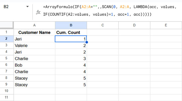
Assume you have the following names in A2:A in Google Sheets:

Jeri
Valerie
Jeri
Charlie
Bob
Charlie
Stacey
Stacey

In cell B2, enter the following formula to get the cumulative count of distinct names:

=ArrayFormula(IF(A2:A="",,SCAN(0, A2:A, LAMBDA(acc, values, IF(COUNTIF(A2:values, values)=1, acc+1, acc)))))

Result:

Formula Explanation

• COUNTIF(A2:values, values) – Returns the running count of occurrences of the current row’s value. This is equivalent to entering =COUNTIF($A$2:A2, A2) in B2 and dragging it down.
• In this COUNTIF, values represents the current value/reference.
• IF(COUNTIF(A2:values, values) = 1, acc + 1, acc) – If the count of values is 1, the formula adds 1 to the accumulator (acc); otherwise, it retains the previous count.
• The SCAN function iterates this logic for each value in the array, returning the running count of distinct values in Google Sheets.
• The IF statement at the beginning ensures that empty rows do not display any result.

Resources

• Filter Distinct Records in Google Sheets
• Distinct Values in Drop-Down List in Google Sheets
• Highlighting Distinct and Unique Values in Google Sheets
• Count Distinct Values in Google Sheets Pivot Table
• Running Count in Google Sheets: Formula Examples
• Reverse Running Count Simplified in Google Sheets
• Fix Interchanged Names in Running Count in Google Sheets
• Running Count of Occurrences in Excel (Includes Dynamic Array)
• Case-Sensitive Running Count in Google Sheets
• Running Count with Structured References in Google Sheets