In this post, let’s explore how to code an array formula for a conditional running total (conditional cumulative sum) in Google Sheets. I have also included a guide on incorporating a group-wise running total in this tutorial.
Previously, for the array formula running total (also known as CUSUM), we were limited to using functions such as SUMIF or MMULT in Google Sheets, whereas Excel allowed the use of MMULT.
However, until recently, the only function suitable for a conditional running total array formula in Google Sheets, to the best of my understanding, was MMULT. Now, with emerging solutions, Lambda functions offer additional possibilities.
The primary focus of this post is the Conditional Running Total (conditional CUSUM) Array Formula in Google Sheets.
I’ve presented two types of examples.
In one example, I’ll illustrate the group-wise running total, indicating separate CUSUM calculations for each group or unique values.
The other example demonstrates how to exclude specific values from the running total (CUSUM).
Furthermore, we can address these two issues using MMULT or Lambda helper functions. Let’s begin with MMULT.
Group-Wise Running Total Array Formula in Google Sheets – MMULT
Key Feature: Works with both sorted and unsorted data.
We have sample data in cells A2:B, where A2:B2 contains the headers. To access the sample data, kindly replicate my sample sheet by clicking the button below.
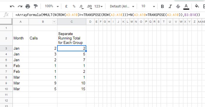
Let’s create the conditional CUSUM formula in cell C3, specifically in the column ‘Separate Running Total for Each Group.’
There are three groups or unique values in the above dataset (refer to column A): Jan, Feb, and Mar.
Although the group column A is sorted, it’s worth noting that even if the data is not sorted group-wise as shown above, my MMULT formula will still work. In other words, the month names can be in any order.
Formula:
=ARRAYFORMULA(IF(LEN(A3:A), MMULT(
     N(ROW(A3:A)>=TRANSPOSE(ROW(A3:A)))*N(A3:A=TRANSPOSE(A3:A)),
     N(B3:B)
),))
Formula Explanation
Note: The formula utilizes the ranges A3:A and B3:B (open ranges). We will test the formula in A3:A10 and B3:B10 (closed ranges).
The above conditional (group-wise) running total array formula in Google Sheets comprises three parts.
The first two parts form matrix 1, and the third part forms matrix 2.
MMULT Syntax: MMULT(matrix1, matrix2)
The conditions must be applied in matrix 1. This is what I’ve done, and I’ve explained the process below.
PART 1 (the first condition in the running total formula)
We aim to calculate a running total with specified conditions. The following segment of the formula generates a matrix for this purpose.
N(ROW(A3:A10)>=TRANSPOSE(ROW(A3:A10)))This Part 1 formula, when used with ArrayFormula, produces the following matrix values.
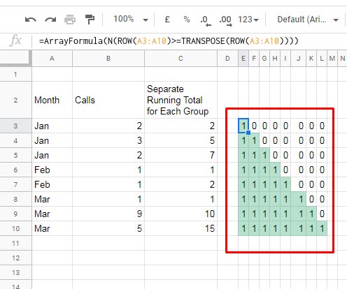
Let me elaborate on this formula:
The ROW(A3:A10) (utilizing ArrayFormula) yields vertical sequence numbers from 3 to 10.
When we transpose this formula using TRANSPOSE(ROW(A3:A10)) (with ArrayFormula), the numbers are returned in a horizontal arrangement.
The formula then checks whether each value in the vertical sequence numbers is equal to its transposed value (horizontal sequence numbers) and returns TRUE or FALSE.
The function N converts TRUE to 1 and FALSE to 0, as illustrated in the image above.
PART 2 (the second condition in the running total formula)
We aim to calculate a group-wise running total, and this part helps us specify that group.
N(A3:A10=TRANSPOSE(A3:A10))This Part 2 formula, when used with ArrayFormula, produces the following matrix values.
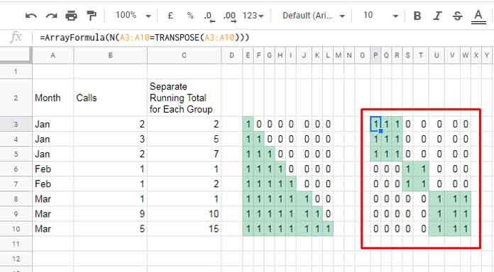
The formula tests whether the values in A3:A10 are equal to the transposed values in A3:A10 and returns TRUE or FALSE. I have converted these Boolean values to 1 or 0 (numbers) using the function N.
So, Part 1 * Part 2 is equal to matrix 1 in the MMULT, which is crucial for obtaining the conditional running total in Google Sheets.
N(ROW(A3:A10)>=TRANSPOSE(ROW(A3:A10)))*N(A3:A10=TRANSPOSE(A3:A10))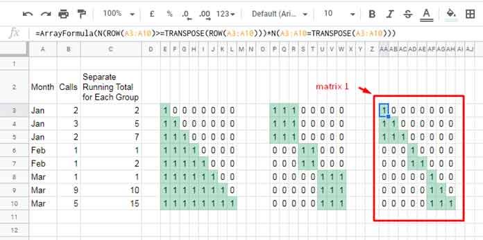
PART 3
Matrix 2 is the range B3:B10 itself.
N(B3:B10)In matrix 2, the purpose of the function N is not to convert TRUE or FALSE to 1 or 0, as there are no TRUE or FALSE values in the range.
Here, it converts blank cells, if any, to 0 to avoid errors in MMULT (since MMULT parameters 1 and 2 require numeric values).
The entire formula is wrapped in an IF and LEN combination. It checks whether the length of the corresponding cell in column A is greater than 0. If true, it calculates the MMULT result; otherwise, it returns an empty result.
That concludes the explanation of the group-wise running total, a type of conditional running total in Google Sheets.
Group-Wise Running Total Array Formula in Google Sheets – BYROW
Key Feature: Works with both sorted and unsorted data.
The above MMULT formula may lead to performance issues with large datasets.
Here is an alternative solution for a group-wise running total in Google Sheets using the BYROW function.
Insert the following formula in cell C3, which will expand down:
=BYROW(A3:A, LAMBDA(r, IF(r="", ,SUM(FILTER(B3:B, A3:A=r, ROW(A3:A) <= ROW(r))))))Note: Feel free to replace BYROW with MAP in the formula above.
Formula Breakdown
FILTER(B3:B, A3:A=r, ROW(A3:A) <= ROW(r)): The FILTER function filters B3:B where A3:A is equal to r, and the row number of A3:A is less than or equal to the row number of r.
Here, r represents the current cell in each row in A3:A. In the first row, A3:A=r will be A3:A=A3, the second row A3:A=r will be A3:A=A4, and so on.
The same logic applies to ROW(A3:A) <= ROW(r). Here, too, r will be A3, A4, and so on for each row. The BYROW function helps iterate through each row in A3:A as above.
IF(r="", ,SUM(FILTER(B3:B, A3:A=r, ROW(A3:A) <= ROW(r)))): The IF function returns the sum of the filtered values in each row if r is not blank.
Conditional Running Total Array Formula in Google Sheets – MMULT
Let’s start with new sample data in the range A2:B (you can get it from my sample sheet shared above).
In the sample data (monthly expense break-up), we want to apply a conditional running total array formula in cell C3.
If we insert the standard running total array formula without condition in cell C3, it would return a wrong cumulative sum (CUSUM).
=ARRAYFORMULA(IF(LEN(A3:A), MMULT(
     IF(ROW(B3:B)>=TRANSPOSE(ROW(B3:B))=TRUE, 1, 0),
     N(B3:B)
),))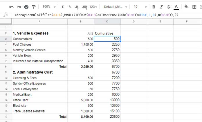
Note: To understand this formula, you can refer to the explanations for PART 1 and PART 3 in our group-wise running total array formula example. Part 1 corresponds to matrix 1, and Part 3 corresponds to matrix 2 in MMULT.
I want to exclude the “Total” rows and the account head row (2. Administrative Cost) from being considered in the running sum (cumulative sum).
Adding Conditions to Running Total Array Formula
Modification 1 (to exclude Total and Subheading rows from the output):
In the formula provided above, replace:
IF(LEN(A3:A)with:
IF((A3:A<>"Total")*(NOT(ISNUMBER(LEFT(A3:A,1)*1)))This modification checks if A3:A doesn’t contain the string “total” and the first character in any string is not a number. If the first character is a number, it means the row contains a subheading, which we want to exclude.
Modification 2 (to exclude “Total” row values in the cumulative sum):
Replace matrix 2, which is:
N(B3:B)with;
IF(A3:A<>"Total", N(B3:B), 0)Here is the much-awaited conditional running total array formula to use in cell C3.
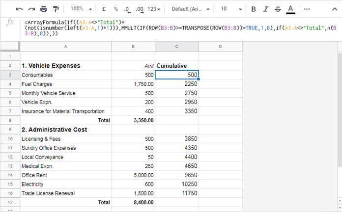
=ARRAYFORMULA(IF((A3:A<>"Total")*(NOT(ISNUMBER(LEFT(A3:A,1)*1))), MMULT(
     IF(ROW(B3:B)>=TRANSPOSE(ROW(B3:B))=TRUE, 1, 0),
     IF(A3:A<>"Total", N(B3:B), 0)
),))
Conditional Running Total Array Formula in Google Sheets – SCAN
Here as well, the purpose of this MMULT alternative is to improve performance.
You can enter the following formula in cell C3:
=ARRAYFORMULA(IF((A3:A="Total")+(B3:B=""), ,SCAN(0, A3:A, LAMBDA(a, v, IF(v="Total", a, OFFSET(v, 0,1 )+a)))))This formula utilizes the SCAN function in Google Sheets for iterative calculations. Here’s the explanation:
SCAN(0, A3:A, LAMBDA(a, v, …): The SCAN function iterates over the values in the range A3:A, applying the Lambda function for each element. The Lambda function takes two parameters:a(accumulator) andv(current value).IF(v="Total", a, OFFSET(v, 0, 1)+a): This is the core logic of the Lambda function. It checks if the current row value (v) is equal to “Total”. If true, it returns the accumulator (a), effectively skipping the “Total” row. If false, it adds the current value (v) in the next column(OFFSET(v, 0, 1))to the accumulator(a).
So, the entire formula effectively calculates a running total, excluding rows where the value in column A is “Total.”
The SCAN returns values in all rows in the array even though it doesn’t use the “Total” row values for calculations. Therefore, we have wrapped the formula with an IF logical test to exclude values from those rows.
This way, you can add other conditions/criteria to the running sum. Thanks for staying tuned, enjoy!
Resources
- Running Total with Monthly Reset in Google Sheets (Array Formula).
- Reset Running Total at Every Year Change in Google Sheets (SUMIF Based).
- Running Count of Multiple Values in a List in Google Sheets.
- Running Count in Google Sheets – Formula Examples.
- How to Calculate Running Balance in Google Sheets.


Hi Prashanth, can the BYROW implementation be applied to a calculated field in a pivot table?
It depends on the use case.
MMULT Formula is very, very slow. It hangs the entire sheet.
Hi, Pankaj Jain,
That’s true! It’ll work only for a small dataset.
Did you check my recent tutorial Reset Running Total at Every Year Change in Google Sheets (SUMIF Based)?
That may help you code a new formula for your need. If not, please share the URL of a sample sheet below. I’ll try to write one.
Hi,
Thank you so much. It works.
Hi Prashanth,
I manage to get that successfully.
However, I have another issue that is indirectly related to this. I have no idea how to transfer 3 columns of query data into a matrix table.
Hi, Desmond Lee,
I could lay my hands on your shared Sheet, but it’s not opening fully. I think the problem is with the “Ranking Table” sheet.
Empty that tab, then enter the below formula in cell A1.
=query('Line Wkly'!A1:G,"Select B,min(E) where B is not null group by B pivot A")Hi There,
If I modify the formula to this –
=ArrayFormula(MMULT(N(ROW(A2:A)>=TRANSPOSE(ROW(A2:A)))*N(A2:A=TRANSPOSE(A2:A)),N(B2:B)))
it shows me the error “Error The resulting array was too large.”
Is there a way to tweak it to run in a larger range?
Hi, Desmond Lee,
It’s because of TRANSPOSE. I have got an alternative solution using a helper range.
Please see the tab “separate CUSUM for groups – larger range” on the shared Sheet.
I have left some notes there.