I’ve two array formulas to get running total with monthly reset in Google Sheets. We can use SUMIF or the SCAN Lambda for this.
But my Lambda Helper Function (LHF) formula requires a helper column, whereas the SUMIF doesn’t.
There may be other options. But I’m sticking with these two because they do not seem to slow down or freeze your Sheet.
Even so, I suggest you use closed ranges such as A2:A100 instead of A2:A in your formula to improve the formula response.
Please note the following.
- Assume you have data spread across years. In that case, the running total will reset at year change also. That means the formula will treat January in 2022 and January in 2023 as two different entities.
- The formula requires sorted data. So you must sort the data based on the date column in ascending (A-Z) order.
Sample Data:
| Date (dd/mm/yy) | Amount | Running Total with Monthly Reset |
| 1/1/22 | 6 | 6 |
| 5/1/22 | 4 | 10 |
| 25/2/22 | 1 | 1 |
| 28/2/22 | 15 | 16 |
| 16/12/22 | 10 | 10 |
| 24/12/22 | 5 | 15 |
| 16/2/23 | 7 | 7 |
| 17/2/23 | 8 | 15 |
| 18/2/23 | 1 | 16 |
| 26/10/23 | 6 | 6 |
SUMIF for Running Total with Monthly Reset
The table range is B1:C11, dates in B2:B11, and amounts in C2:C11 (please scroll down to see the image with sample data).
In that range, cells B1, C1, and D1 contain the column names “Date (dd/mm/yy),” “Amount,” and “Running Total with Monthly Reset.”
Insert the following SUMIF formula in cell D2.
=ArrayFormula(if(len(B2:B),sumif(row(B2:B), "<="&row(B2:B), C2:C)-sumif(eomonth(B2:B,0), "<"&eomonth(B2:B,0), C2:C),))It will return the running total that resets w.r.t. every month change in column B.
Do you want to know how the above running total with the monthly reset array formula works? Here you go!
Anatomy of the Formula
It’s so simple to learn if you peel the formula. You will get three parts if you do it properly.
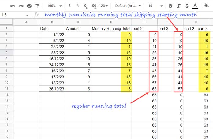
- Part_1 (Highlighted in Vivid Green Cyan color)
- Part_2 (Highlighted in Vivid Red color)
- Part_3 (Highlighted in Vivid Purple color)
The role of Part_1 LEN and IF combo is to help the running total monthly reset formula to identify blank rows after row#11 and exclude calculations in that row. It works like if(len(B2:B), do this, ,)
Part_2 returns the regular running total of column C.
=ArrayFormula(sumif(row(B2:B), "<="&row(B2:B), C2:C))What does the Part_3 formula do?
I’ll come to that.
If you modify < to <= in the criteria part of the Part_3 formula, it will return the monthly cumulative running total.
=ArrayFormula(sumif(eomonth(B2:B,0), "<="&eomonth(B2:B,0), C2:C))So you will get the January total in all the January rows, the January total + February total in all the February rows, and so on.
If we remove the equal sign, the formula will skip the result one month down.
Part_2 – Part_3 = Running Total that Resets when Month Changes.

SCAN LHF for Running Total with Monthly Reset
I suggest the above array formula to return the running total with the monthly reset in Google Sheets.
This SCAN approach is to help you learn this LAMBDA helper function as it’s relatively new.
This approach involves three steps and two formulas.
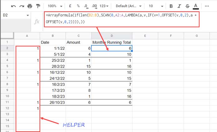
- Inserting a regular running count formula in cell A1.
- Converting running count output >1 to blank by modifying the same formula in cell A1.
- The SCAN formula in cell D2 that returns the running total that resets at every month change row.
Here are those three steps and two formulas.
Insert the following formula in cell A1.
=ArrayFormula(countifs(row(B2:B),"<="&row(B2:B),eomonth(B2:B,0),eomonth(B2:B,0)))It returns the running count of months. Edit it as below to replace all the values >1 in the output with blank.
=ArrayFormula(if(countifs(row(B2:B),"<="&row(B2:B),eomonth(B2:B,0),eomonth(B2:B,0))>1,,1))
Finally, enter the following SCAN formula in cell D1, and voila!
=ArrayFormula(if(len(B2:B),SCAN(0,A2:A,LAMBDA(a,v,IF(v=1,OFFSET(v,0,2),a + OFFSET(v,0,2)))),))Here the SCAN LHF works like this. If the value (v) in column A is 1, it offsets two columns and returns the value in that cell.
Else it offsets two columns and returns the value in that cell + accumulator value (a).
You May Like: Custom Named Function for Running Total by Group (Item, Month, or Year) In Google Sheets.


