How to get the count of occurrences of values in each row in Google Sheets?
Here get an array formula equivalent to drag and drop Countif formula. A useful Google Sheets formula, if you want to count occurrences of items in each row in a dataset in Google Sheets.
First of all, let me introduce to you a sample dataset and then the Countif drag and drop formula. That will be easy for me to explain the topic and for you to understand what I have meant.
Find the sample data and the non-array formula below.
Countif Non-Array Formula to Get Count of Occurrences in Each Row in Google Sheets
The Countif formula in cell C2 counts the occurrences of the value (name) in cell B2 in the range B2:B11.
=countif(B2:B11,B2)When dragging the formula down, the range to count as well as the criterion changes. For example, in cell B3 the criterion will be from cell B3 and the range will be B3:B12.
Screenshot # 1:
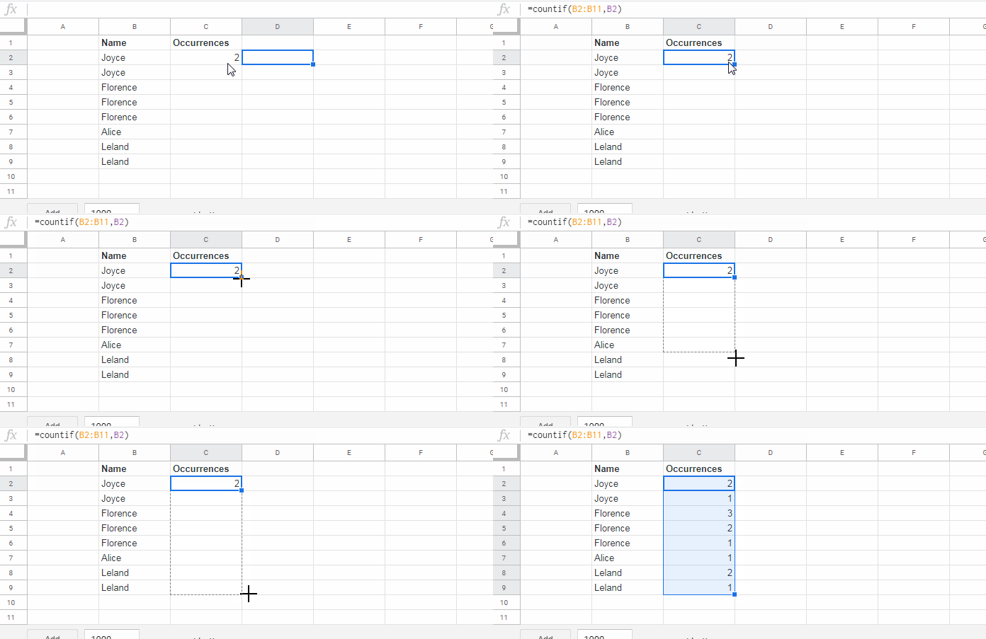
That means the Countif formula counts the occurrence of values in the range starting from the row it keyed in.
Even though the Countif formula above is very simple, it has the drawbacks of drag and drops formula as below.
- Either you need to copy-paste the formula to the whole column (C2:C) or copy-paste as and when new rows are added to the data set.
- If you insert a row in the existing range, you may need to copy-paste the formula from the cell above to the adjoining cell in the new row inserted.
I have an array formula to count occurrences in each row as an alternative to the Countif above in Google Sheets.
The formula may seem complex to you. But you can forget about the formula and logic and use it out of the box.
For those who are interested, I will include the explanation below.
Array Formula to Get the Count of Occurrences of Values in Each Row
The Formula in C2:
=ArrayFormula(array_constrain(sort({COUNTIFS(index(sort({B2:B,row(B2:B)},2,0),0,1),index(sort({B2:B,row(B2:B)},2,0),0,1),ROW(A2:A),"<="&ROW(A2:A)),sort({B2:B,row(B2:B)},2,0)},3,1),match(2,1/(B1:B<>""))-row(B1),1))Formula Logic: Reversing Running Count
Update: I have a new simple formula to replace the above one. You can find that here – Reverse Running Count Simplified in Google Sheets.
To make you understand the logic of the above combination formula which returns the count of occurrences of values in each row in Google Sheets, you must see this running count output.
For explanation purposes, I have marked the running count of the name “Florence”.
Screenshot # 2:
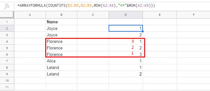
If we can reverse the running count we will get the count of occurrence of the name ‘Florance’ like the Countif does (please refer to Screenshot # 1) such as 3, 2, 1 instead of 1, 2, 3.
Reversing the running count is the logic that I have used in my array formula which returns the count of occurrences in each row.
Let’s see how to reverse the running count formula in Google Sheets under the formula explanation below.
Explanation – How the Formula Counts the Occurrence in Each Row?
I will only use a limited range in the explanation. I mean the range will be a closed range, i.e. B2:B9 instead of B2:B.
Once complete, we can make the reference open. There are three steps involved/to follow in this explanation part. They are;
- Flip Data from Bottom to Top.
- Running Count of Flipped Column.
- Reverse Flipping.
Flipping Data from Bottom to Top
First, make a two-column array using Curly Brackets. The first column contains the existing names in B2:B9 and the second column contains row numbers from 2 to 9.
=ArrayFormula({B2:B9,row(B2:B9)})Then sort the second column in descending order. That’s what the below formula does.
Here is the formula that I have used to flip the data from bottom to top (removed ArrayFormula. Not required with SORT).
Formula # 1:
=sort({B2:B9,row(B2:B9)},2,0)Screenshot # 3:
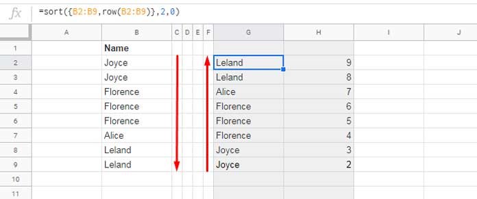
This has been already featured in my earlier tutorial – How to Flip a Column in Google Sheets – Finite and Infinite Columns.
Finding Running Count of Flipped Column
Key this running count formula in cell F2 which returns the running count of the flipped names in column G.
=ARRAYFORMULA(COUNTIFS(G2:G9,G2:G9,ROW(A2:A9),"<="&ROW(A2:A9)))Note: Running count has been explained here – Running Count in Google Sheets – Formula Examples.
Screenshot # 4:
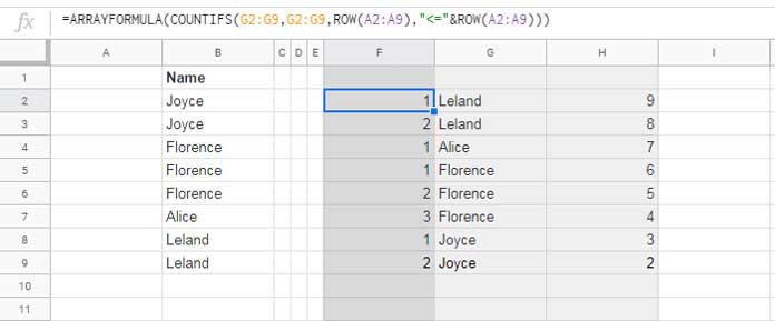
You can replace G2:G9 (twice) in the formula with formula 1. Formula 1 returns two columns in the range G2:H9, right? But we just want the values in G2:G9.
So using Index we can extract the first column only from the formula 1 result.
Generic Formula:
=index(formula 1,0,1)Here is the formula.
=index(sort({B2:B9,row(B2:B9)},2,0),0,1)We can now modify the formula in cell F2 as below.
Formula # 2:
=ARRAYFORMULA(COUNTIFS(index(sort({B2:B9,row(B2:B9)},2,0),0,1),index(sort({B2:B9,row(B2:B9)},2,0),0,1),ROW(A2:A9),"<="&ROW(A2:A9)))Now combine the above formulas 1 and 2. It would be like;
={formula 1,formula 2}Here is the combined formula in F2.
Formula # 3:
={ARRAYFORMULA(COUNTIFS(index(sort({B2:B9,row(B2:B9)},2,0),0,1),index(sort({B2:B9,row(B2:B9)},2,0),0,1),ROW(A2:A9),"<="&ROW(A2:A9))),sort({B2:B9,row(B2:B9)},2,0)}Don’t forget to remove the formula in cell G2 to expand this formula output to column G2:H.
After applying the above formula, we will have the data as per screenshot 4 above.
Now we only need to do reverse the flipping and remove the second and third columns (column G and H). So that we will get the count of occurrences of names in each row in Google Sheets.
Reverse Flipping
To reverse flip, sort the third column contains row numbers (in the F2 formula output) in ascending order.
Generic Formula:
=sort(Formula 3,3,1)Here are the reversing flipping formula and its output.
Formula # 4:
=sort({ARRAYFORMULA(COUNTIFS(index(sort({B2:B9,row(B2:B9)},2,0),0,1),index(sort({B2:B9,row(B2:B9)},2,0),0,1),ROW(A2:A9),"<="&ROW(A2:A9))),sort({B2:B9,row(B2:B9)},2,0)},3,1)Screenshot # 5:
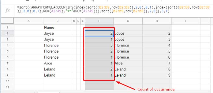
We just want the first column F2:F9 which returns the count of occurrence in each row, right?
Final Steps:
First of all, make the ranges in the formula open. To do that change B2:B9 to B2:B and A2:A9 to A2:A.
Formula # 5:
=sort({ARRAYFORMULA(COUNTIFS(index(sort({B2:B,row(B2:B)},2,0),0,1),index(sort({B2:B,row(B2:B)},2,0),0,1),ROW(A2:A),"<="&ROW(A2:A))),sort({B2:B,row(B2:B)},2,0)},3,1)Screenshot # 6:
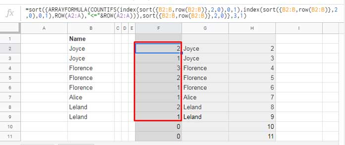
This open range fills 0s at the end of the range in column F. We can control the formula to only fill occurrences in F10:F if there are values in B10:B.
Let’s use Array_constrain function to extract the count of occurrences within the marked range. How?
Generic Formula:
=Array_Constrain(Formula 5,8,1)In this generic formula, 8 represents the number of rows to return (the counts of rows in the range B2:B9) and 1 represents the column.
Here is the issue. We know we want 1 column. But what about rows?
We can dynamically find the row count (8) in the range B2:B by using this formula.
=ArrayFormula(match(2,1/(B1:B<>""))-row(B1))So we can modify the above generic formula by replacing the row count 8 with the above formula as below.
=Array_Constrain(Formula 6,ArrayFormula(match(2,1/(B1:B<>""))-row(B1)),1)Final Formula in Cell C2:
=Array_Constrain(sort({ARRAYFORMULA(COUNTIFS(index(sort({B2:B,row(B2:B)},2,0),0,1),index(sort({B2:B,row(B2:B)},2,0),0,1),ROW(A2:A),"<="&ROW(A2:A))),sort({B2:B,row(B2:B)},2,0)},3,1),ArrayFormula(match(2,1/(B1:B<>""))-row(B1)),1)You can remove the two ArrayFormula functions within and use only one at the beginning.
That’s all.
I hope, I have well explained how to get the count of occurrences in each row using an array formula in Google Sheets.
Thanks for the stay. Enjoy!


Hi Prashanth,
May I get the formula for the same without the reversing? I would like to get 1,2,3.. instead of reverse order.
Thanks,
Saravanan N K
Hi, Saravanan N k,
Replace B2:B with your actual range.
=ArrayFormula(let(rc,COUNTIFS(B2:B,B2:B,ROW(B2:B),"<="&ROW(B2:B)),if(rc=0,,rc)))Prashanth,
Not sure what you’re trying to get with your arrayformula.
Have you tried;
1) either us relative/absolute markers in your formulas? Dragging or copy/pasting will actually work if you use a simple
=COUNTIF($D$26:$D$33;$D26)2) or use a very simple Arrayfomula such as
=ARRAYFORMULA(COUNTIF(D26:D33;D26:D33))Both give the same result, and are not too complex 🙂
Hi, Frank Oers,
The difference in cumulative aka running count.
If an item, for example, “book” repeated 5 times, in each row your formula would return 5. But mine would 1, 2,…5.