Reversing an array, whether it’s 1D or 2D, can be tricky in Google Sheets, and the formula depends on the direction of the data.
If you want to flip a vertical array from bottom to top, you’ll need one formula, while flipping from right to left requires another.
Formula to Reverse a Vertical Array in Google Sheets (Flip Bottom to Top)
=ArrayFormula(CHOOSEROWS(range, SEQUENCE(XMATCH(TRUE, CHOOSECOLS(range, 1)<>"", 0, -1), 1, XMATCH(TRUE, CHOOSECOLS(range, 1)<>"", 0, -1), -1)))range – The 1D or 2D array you want to flip from bottom to top.
Formula to Reverse a Horizontal Array in Google Sheets (Flip Right to Left)
=ArrayFormula(CHOOSECOLS(range, SEQUENCE(XMATCH(TRUE, CHOOSEROWS(range, 1)<>"", 0, -1), 1, XMATCH(TRUE, CHOOSEROWS(range, 1)<>"", 0, -1), -1)))range – The 1D or 2D array you want to flip from right to left.
Features of the Reverse Array Formula
Reversing an Array Vertically:
- Works with both closed and open ranges, e.g.,
A1:C100orA1:C(open-ended rows). - Trims empty rows from the end.
- Retains blank rows in the middle.
- Uses the first column to determine the last used row.
- Works for single or multiple columns.
Reversing an Array Horizontally:
- Works with both closed and open ranges, e.g.,
A1:C100orA1:100(open-ended columns). - Trims empty columns from the end.
- Retains blank columns in the middle.
- Uses the first row to determine the last used column.
- Works for single or multiple rows.
Reverse a Vertical Array (Single or Multiple Columns)
To understand how to reverse an array in Google Sheets, let’s consider a real-life example.
We have the following table in A1:D13, where column A lists months (Jan to Dec), and columns B, C, and D contain sales data for three items.
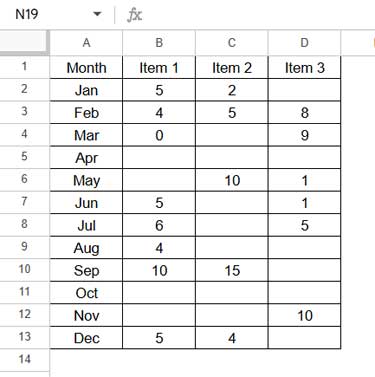
By reversing this array vertically, we bring the latest sales data to the top, sorting from Dec to Jan.
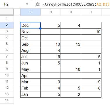
Formula to Reverse the Array Vertically
=ArrayFormula(CHOOSEROWS(A2:D13, SEQUENCE(XMATCH(TRUE, CHOOSECOLS(A2:D13, 1)<>"", 0, -1), 1, XMATCH(TRUE, CHOOSECOLS(A2:D13, 1)<>"", 0, -1), -1)))This formula reverses the array. If you want to accommodate future entries, use an open range like A2:D.
Output:
Formula Breakdown
The formula primarily uses the CHOOSEROWS function to reorder rows dynamically.
For example:
=CHOOSEROWS(A2:D13, {12, 11, 10, 9, 8, 7, 6, 5, 4, 3, 2, 1})This manually reverses the array.
To generate row numbers dynamically, we use:
SEQUENCE(XMATCH(TRUE, CHOOSECOLS(A2:D13, 1)<>"", 0, -1), 1, XMATCH(TRUE, CHOOSECOLS(A2:D13, 1)<>"", 0, -1), -1)Syntax:
SEQUENCE(rows, [columns], [start], [step])Where:
- rows:
XMATCH(TRUE, CHOOSECOLS(A2:D13, 1)<>"", 0, -1)– Finds the last used row. - columns:
1– Number of columns in the sequence. - start: Same as the
rowsargument, dynamically determining the starting row number. - step:
-1– Generates the sequence in descending order.
Since the formula determines the last used row based on the first column, it reverses the array from that point to the first row.
Reverse a Horizontal Array (Single or Multiple Rows)
Now, let’s see how to reverse an array horizontally.
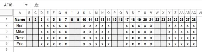
Consider a dataset with names in column A and attendance records in columns B:AC (1/2/2025 to 28/2/2025).
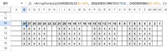
Formula to Reverse the Array Horizontally
=ArrayFormula(CHOOSECOLS(B2:AC5, SEQUENCE(XMATCH(TRUE, CHOOSEROWS(B2:AC5, 1)<>"", 0, -1), 1, XMATCH(TRUE, CHOOSEROWS(B2:AC5, 1)<>"", 0, -1), -1)))This flips the array horizontally.
Formula Explanation:
- Uses CHOOSECOLS instead of CHOOSEROWS to reorder columns.
- Uses CHOOSEROWS to extract the first row to determine the last column.
Why Reverse an Array in Google Sheets?
Flipping arrays, whether horizontally or vertically, serves one major purpose: Easier access to the latest data.
Since data is typically entered top-to-bottom or left-to-right, recent entries end up at the bottom or far right. Reversing the array brings the latest data to the top or left, making it more accessible.
You can also combine this formula with QUERY, ARRAY_CONSTRAIN, VLOOKUP, etc., to manipulate recent data effectively.


=transpose(arrayformula(Sheet!1:1) )