You can reverse text and numbers in Google Sheets in two main ways. One approach uses split and transpose, while the other extracts each character or digit from the end. In both methods, we combine the extracted values to form the reversed result.
Approach 1 Formula
=TEXTJOIN(
   "",
   TRUE,
   CHOOSECOLS(
      SPLIT(REGEXREPLACE(A1&"", ".", ",$0"), ","),
      SEQUENCE(LEN(A1), 1, LEN(A1), -1)
   )
)- For reversing text and numbers.
Approach 2 Formula
=ARRAYFORMULA(
   TEXTJOIN(
      "",
      TRUE,
      MID(A1, SEQUENCE(LEN(A1), 1, LEN(A1), -1), 1)
   )
)- For reversing text, numbers, dates, and datetime.
Replace A1 with the cell containing the text or number to reverse.
Explanation of the Formulas to Reverse Text and Numbers in Google Sheets
I’ve mentioned two approaches, and here’s the detailed breakdown of how they work:
Approach 1: Using REGEXREPLACE, SPLIT, and CHOOSECOLS
REGEXREPLACE(A1&"", ".", ",$0")
This function, i.e., REGEXREPLACE, separates each character in the value by inserting a comma before it.
Example:"Sheets"becomes",S,h,e,e,t,s".SPLIT(..., ",")
The SPLIT function splits this comma-separated string into individual columns.
Example:",S,h,e,e,t,s"becomes{"S", "h", "e", "e", "t", "s"}.CHOOSECOLS(..., SEQUENCE(LEN(A1), 1, LEN(A1), -1))
Here, CHOOSECOLS selects the columns in reverse order because the SEQUENCE function generates numbers in descending order, starting from the length of the value inA1down to 1.
Example: The characters are rearranged as{"s", "t", "e", "e", "h", "S"}.TEXTJOIN("", TRUE, ...)
Finally, TEXTJOIN combines these reversed characters into a single string.
Example:"steehS".
Approach 2: Extracting Characters from the End Using MID
This is the most common approach among spreadsheet users for reversing text and numbers because the functions used are familiar to most users.
SEQUENCE(LEN(A1), 1, LEN(A1), -1)
This creates a sequence of numbers starting from the last character’s position and ending with the first.
Example: For"Sheets", it generates{6, 5, 4, 3, 2, 1}. We’ve seen this sequence in the first approach as well.MID(A1, SEQUENCE(...), 1)
The MID function extracts one character at a time based on the sequence.
Example: Extracts"s","t","e","e","h","S".TEXTJOIN("", TRUE, ...)
Combines the extracted characters into a single reversed string.
Example:"steehS".- ARRAYFORMULA
This ensures the formula works for multiple cells in a range if applied to an array.
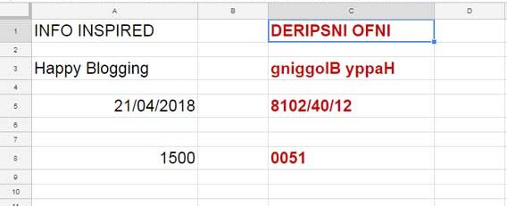
Reverse Text and Numbers in a Column (Array Formula)
If you have values in the range A1:A, you can apply one of the formulas mentioned earlier in cell B1 and drag it down to reverse all values. However, you can use the MAP function with a LAMBDA helper function to automate this process.
Generic Formula:
=IFERROR(MAP(A1:A, LAMBDA(row, formula_here)))Replace formula_here with one of the formulas we used earlier to reverse text and numbers. In these formulas, replace the cell reference A1 with the variable name row.
For example, the formula in cell B1 will be:
=IFERROR(MAP(A1:A, LAMBDA(row,
   ARRAYFORMULA(
      TEXTJOIN(
         "",
         TRUE,
         MID(row, SEQUENCE(LEN(row), 1, LEN(row), -1), 1)
      )
   )
)))
Related Resources
If you’re interested in similar topics, check these out:
- How to Flip a Column in Google Sheets – Finite and Infinite Columns
- Flip a Table Vertically in Excel (Includes Dynamic Array Formula)
- How to Reverse an Array in Google Sheets (Fixed and Dynamic Array)
Both approaches are simple to use. Pick the one that works best for you!


