Effortlessly automate your running balance calculations in Google Sheets using either the SUMIF or SCAN functions.
Both formulas are included in this tutorial, providing clear explanations and practical examples. You’ll master both methods and choose the one that best fits your needs.
The SUMIF and SCAN-based solutions are array formulas that you can set and forget, automatically updating with each new transaction.
For those who prefer a drag-down formula, especially beginners, I’ve included that option as well.
What is a running balance?
A running balance is a dynamic calculation. It reflects the cumulative balance of an account or financial transactions over time. This balance updates with each new transaction, capturing the total amount after each addition or subtraction.
For example purposes, we’ll use a sample bank statement with separate debit and credit columns and guide you through creating running balance formulas (both array and non-array) in a third column.
We’ll then show you how to handle situations where both debit and credit are in the same column, ensuring you have the flexibility to handle any scenario.
Non-Array Running Balance Formula in Google Sheets (Debit and Credit Transactions in Separate Columns)
Examine the sample data provided in cell range A1:D12:
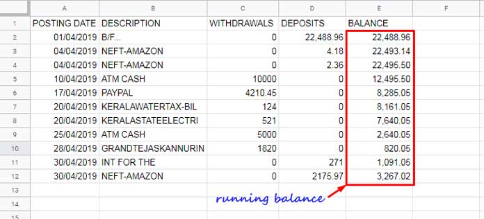
Column A contains transaction dates, B has descriptions, and C and D record withdrawals (debit) and deposits (credit), respectively.
To calculate the running balance in column E, we’ll use data from columns C and D.
We’ll begin with a non-array (drag-down) formula and later explore the SUMIF and SCAN solutions.
First, enter the following formula in cell E2:
=SUM($D$2:D2)-SUM($C$2:C2)Drag down the formula (use the fill handle) until it reaches cell E12.
In each row, the running balance is calculated.
It involves subtracting the cumulative sum of withdrawals from the cumulative sum of deposits, starting from the initial balance. This is achieved using a combination of relative and absolute cell references.
The formula will automatically adjust to become =SUM($D$2:D3) - SUM($C$2:C3), =SUM($D$2:D4) - SUM($C$2:C4), and so on.
This is because one part of the cell reference is an absolute cell reference (denoted by the dollar sign), and the other part is relative.
Related: Google Sheets: Dollar Symbols and Relative/Absolute References
Array Formulas for Running Balance in Google Sheets (Separate Debit and Credit Columns)
We can use array formulas to calculate the running balance in Google Sheets.
As you may already be aware, an array formula for running balance can populate the result in each row without the need to drag it down.
There are two methods: SUMIF (traditional) and SCAN. The latter is a clean and straightforward formula, but it’s a LAMBDA helper function, so it might not be suitable for very large datasets.
Running Balance: SUMIF Approach
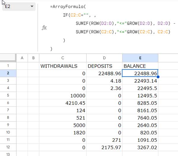
Enter the following formula in cell E2. Ensure there are no blank cells in C2:C in the data range. If any, fill them with 0.
Running Balance Array Formula (SUMIF-Based):
=ArrayFormula(
     IF(C2:C="", ,
          SUMIF(ROW(D2:D),"<="&ROW(D2:D), D2:D) -
          SUMIF(ROW(C2:C),"<="&ROW(C2:C), C2:C)
     )
)
Anatomy of the Formula:
Step #1: The following SUMIF array formula will yield the running total of deposits (D2:D).
=ArrayFormula(SUMIF(ROW(D2:D),"<="&ROW(D2:D), D2:D))Step #2: This will provide the running total of withdrawals (C2:C).
=ArrayFormula(SUMIF(ROW(C2:C),"<="&ROW(C2:C), C2:C))Note: You can learn these formulas from my tutorial titled Normal and Array-Based Running Total Formulas in Google Sheets.
Running balance = Array_Formula(running_total_of_deposits - running_total_of_withdrawals)
When nesting these two (Step #1 and Step #2) array formulas, you need to remove the ArrayFormula function from them, and here it is:
=ArrayFormula(SUMIF(ROW(D2:D),"<="&ROW(D2:D), D2:D) - SUMIF(ROW(C2:C),"<="&ROW(C2:C), C2:C))How do I remove the trailing running balance amounts in the blank rows after the data range?
Immediately after the ArrayFormula(, insert IF(C2:C="", ,.
Running Balance: SCAN Approach
The SCAN is one of the Lambda helper functions used for calculating running totals and balances in Google Sheets. It’s straightforward to use, and here is the formula to use in cell E2:
=ArrayFormula(
     IF(C2:C="", ,
         SCAN(0, D2:D-C2:C, LAMBDA(a, v, IF(v="", ,a+v)))
    )
)
The IF(C2:C="", , is included to avoid the trailing blank cell repeating the last running balance.
What about the SCAN?
Formula Breakdown:
Let’s start with the syntax of the SCAN function:
SCAN(initial_value, array_or_range, lambda)The SCAN iterates over each value in an array, i.e., D2:D-C2:C, and returns the accumulated value in the intermediate calculations using an unknown lambda function.
The lambda function here is IF(v="", , a+v) where ‘a’ represents the accumulated value from the previous iteration, and ‘v’ represents the current value from the combined deposit and withdrawal cell. The initial value in the accumulator is 0.
Calculate Running Balance When Debit and Credit Transactions are in the Same Column
When managing income, expenditure, deposits, withdrawals, etc., within a single column, employ running totals. This will equate to a running balance due to positive and negative amounts in the column.
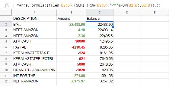
In the sample data shown below, both debit and credit transactions are combined in column B. Negative amounts represent debit/expense/withdrawals, while positive amounts signify credit/income/deposits.
Non-Array Formula:
=SUM($C$2:C2)When dragged down, the formula becomes $C$2:C3, $C$2:C4, and so on.
SUMIF Array Formula:
=ArrayFormula(IF(C2:C="", , SUMIF(ROW(C2:C), "<=" & ROW(C2:C), C2:C)))This is simply a running total formula.
SCAN Array Formula:
=ArrayFormula(IF(C2:C="", , SCAN(0, C2:C, LAMBDA(a, v, IF(v="", ,a+v)))))This formula is similar to calculating the running balance with debit and credit transactions in two separate columns.
The only change is the array. Earlier, we deducted credit and debit in the array like D2:D-C2:C. Here, we specify only the data column.
Resources
Mastered running balance calculations in Google Sheets? It’s time to delve into related resources that discuss running totals with advanced criteria applications.
- Array Formula for Conditional Running Total in Google Sheets
- Reverse Running Total in Google Sheets (Array Formula)
- How to Calculate a Horizontal Running Total in Google Sheets
- Reset Running Total at Every Year Change in Google Sheets (SUMIF Based)
- Running Total by Category in Google Sheets (SUMIF Based)
- Running Total with Monthly Reset in Google Sheets (Array Formula)
- Custom Named Function for Running Total by Group (Item, Month, or Year) In Google Sheets
- Weekly and Biweekly Running Totals in Google Sheets
- Reset Running Total at Blank Rows in Google Sheets
- Running Total with Multiple Subcategories in Google Sheets


I have just started using Google sheets for my finances and have a running balance for different accounts.
I am trying to get the final running balance from each account to show on a table for a quick view of the balance.
Please, can you help me?
Hi, Amanda,
I will try. Feel free to share the URL of a sample Sheet in your reply below.
Hi, I am a fairly new user.
I have set up an income/expense spreadsheet on Google Sheets that tracks my fixed month-to-month expenses, daily expenses, and future bank balances needed on upcoming dates to pay upcoming monthly bills.
I am looking for help in 2 areas.
First, how do I insert a new row for daily expenses that also pastes the formula, and is there a way to populate a certain cell with the expense using a drop-down menu.
Hi, Brian,
Regarding the “new row for daily expenses,” the given formula will automatically include the new row(s).
To help you populate the expense using drop-down, I may want to see your data layout.
If possible, make a sample sheet and share the link below.
As a fairly novice user of using sheets for the petty cash system, I was hitting my head against a brick wall wondering why I couldn’t get it to sum up or provide a running balance. Thank you so much – these formulae are just the job
Great explanation! Is it possible to have excel calculate from a starting amount?
Thank you! That was exactly what I wanted!
I’m almost a complete newbie to Google Sheets/Excel. I was able to figure out how to use this formula to keep a running total on my spreadsheet. Thank you!
I was wondering if I can put that running total in a header row so that you can always see the balance without having to scroll down?
Hi, MaryJane Hewitt,
It depends on the data presented in your Sheet.
If the income is in column C and expenditure is in column D, then you can use the below formula in the header row in any other column.
=sum(C:C)-sum(D:D)If the income and expenditure are in the same column (as positive and negative values), for example in column C, then the formula to use will be;
=sum(C:C)This was extremely helpful formula.
Thank you
Michael D