Google Sheets users are well-acquainted with the powerful XLOOKUP function, making the question of whether to use it over other lookup functions less relevant. Now, it’s time to explore advanced techniques, such as Nested XLOOKUP in Google Sheets.
A nested XLOOKUP formula is incredibly versatile. It can retrieve values from multiple tables by searching through them sequentially or even work within a single table.
Syntax:
XLOOKUP(search_key, lookup_range, result_range, [missing_value], [match_mode], [search_mode])In a nested XLOOKUP in Google Sheets, the second XLOOKUP is typically used in the lookup_range, result_range, or missing_value if only one table is involved. For scenarios involving two tables, the second XLOOKUP is often used to generate the search_key.
Let’s dive into examples to see how it works.
Nested XLOOKUP with One Table
Imagine you’re a birdwatcher maintaining a spreadsheet of your recent encounters with common and rare bird species.
Your data is structured as follows:
- Column A: Weekday
- Column B: Bird Name
- Column C: Number of Views
To find the number of views for “Quail,” you would typically use:
=XLOOKUP("Quail", B2:B, C2:C)This works if you know that the bird names are in Column B and the results are in Column C. But what if you’re unsure which column contains the search key (bird name)?
Example 1: Replacing lookup_range with a Dynamic Formula
Field labels like “Weekday,” “Bird Name,” and “Number of Views” in the top row (A1:C1) are key. Here’s how you can dynamically find the lookup_range:
=XLOOKUP("Bird Name", A1:C1, A2:C)This formula searches for the field label “Bird Name” in the top row and returns the corresponding column. Now, replace B2:B in the earlier formula with this dynamic result:
=XLOOKUP("Quail", XLOOKUP("Bird Name", A1:C1, A2:C), C2:C)If the search keys are in cells E2 and F2, the formula becomes:
=XLOOKUP(F2, XLOOKUP(E2, A1:C1, A2:C), C2:C)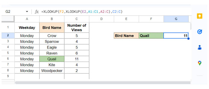
This is a practical example of Nested XLOOKUP in Google Sheets.
Advanced Nested XLOOKUP with Filters
In real-world scenarios, you might need to filter data before applying the nested formula. For instance, to apply the formula only to rows where the weekday is “Monday”:
=LET(range, FILTER(A2:C, A2:A="Monday"), XLOOKUP(F2, XLOOKUP(E2, A1:C1, range), CHOOSECOLS(range, 3)))Here:
- FILTER extracts rows for “Monday.”
- LET assigns a name (“range”) to this filtered data.
- CHOOSECOLS selects the required column (third).
Example 2: Replacing result_range with a Dynamic Formula
For a dataset where Column A contains employee names and Columns B to D represent monthly sales leads, here’s how to find Jennifer’s February sales dynamically:
=XLOOKUP(G2, A2:A, XLOOKUP(H2, A1:E1, A2:E))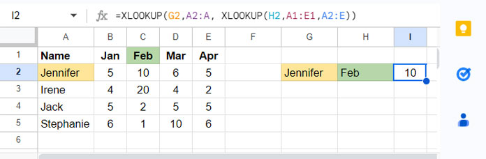
Here:
G2contains the name “Jennifer.”H2specifies the month “Feb.”- The inner XLOOKUP dynamically determines the column for “Feb.”
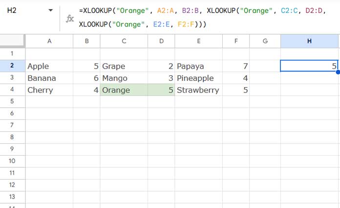
Example 3: Replacing missing_value with a Nested XLOOKUP
A truly nested XLOOKUP in Google Sheets can handle missing values by chaining multiple XLOOKUP functions. For example:
=XLOOKUP("Orange", A2:A, B2:B, XLOOKUP("Orange", C2:C, D2:D, XLOOKUP("Orange", E2:E, F2:F)))This formula searches “Orange” in three lookup-result pairs sequentially, stopping at the first match.
Nested XLOOKUP with Two Tables
For scenarios with multiple tables, one XLOOKUP can generate the search_key for another.
Example 1: Replacing search_key with XLOOKUP
Suppose you have two tables, “emp data” and “salary,” with “ID” as the common field. To find the gross salary of “Ben” using his name:
=XLOOKUP(XLOOKUP("Ben", 'emp data'!B2:B, 'emp data'!A2:A), salary!A2:A, salary!C2:C)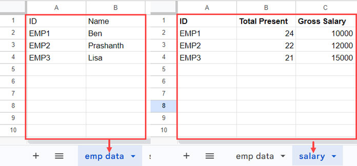
Here:
- The inner XLOOKUP retrieves Ben’s ID from the “emp data” table.
- The outer XLOOKUP uses the ID to fetch Ben’s salary from the “salary” table.
Conclusion
The Nested XLOOKUP in Google Sheets is a robust tool for solving complex lookup scenarios. Whether you’re working within a single table or across multiple tables, mastering this function will elevate your Google Sheets expertise.
If you want to explore more techniques like this, visit our Complete Guide to XLOOKUP in Google Sheets, where we compile practical XLOOKUP examples in Google Sheets ranging from beginner formulas to advanced lookup strategies.


