To search for a key across the first row of a 2D array and return a value from a specified row, use the HLOOKUP function in Google Sheets.
For example, the first row of the range B1:L1000 contains month names, such as “January”, “February”, “March”, and so on. Below that row, we have the corresponding months’ sales volume.
Cell A1 contains the field label “Name”. Below that cell, we have a couple of salesperson’s names. One of the names is “Ben”, and he is in row 6.
You can use the key “February” in the HLOOKUP function to search across the first row and return the value from row 6 to get Ben’s sales volume in February.
On the contrary, to search down the first column for the name “Ben” and return his sales volume from the second column, use the VLOOKUP function.
These two are not the only functions in spreadsheets for lookup operations. There are others like XLOOKUP, LOOKUP, and a combination of the INDEX and MATCH or XMATCH functions.
MATCH and XMATCH are match functions. They find the row or column index of a value in a range of cells. INDEX is an offset function. It returns the value from a cell that is offset by a certain number of rows and columns from a given cell.
In this tutorial, let’s learn how to use the HLOOKUP function in Google Sheets.
HLOOKUP Function: Syntax and Arguments
Syntax of HLOOKUP in Google Sheets:
HLOOKUP(search_key, range, index, [is_sorted])Arguments:
Search_key: The value that you want to find in the first row of the data set. You can either type it directly into the formula or use a cell reference to point to the cell that contains the value.
Range: The range of cells to be considered for the search. Use a reference to a range or a named range.
Index: The row number in the range from which the matching value will be returned.
Is_sorted: A logical value that determines whether the search is for an exact match or the nearest match of the search_key in the first row. It is an optional argument. If you omit it, the formula will use TRUE.
- TRUE (in a sorted range only): The nearest match (approximate match).
- FALSE (in both sorted or unsorted range): An exact match.
When is_sorted is TRUE, if an exact match is not found in the first row, the nearest value less than the search_key is matched.
Search_key Examples in HLOOKUP Function in Google Sheets:
In the table below, you can see how to use text, date, time, and number as search_key within the HLOOKUP function.
| Type of Value | Example | Note |
| Text | “Yumbilla Falls” | |
| Date | DATE(2023, 06, 30) | DATE(year, month, day) |
| Time | TIME(14, 30, 0) | TIME(hour, minute, second) |
| DateTime | DATE(2023, 06, 30)+TIME(14, 30, 0) | DATE(year, month, day)+TIME(hour, minute, second) |
| Number | 1234567890 |
You can also use the search_key as a cell reference. Enter the key in a cell and then refer to that cell in the HLOOKUP function.
Horizontal Lookup in an Unsorted Range
Search_key: “Yumbilla Falls”
Range: A1:J4 (unsorted)
Index: 4
Is_sorted: FALSE
Horizontal Lookup Formula:
=HLOOKUP("Yumbilla Falls",A1:J4,4,false)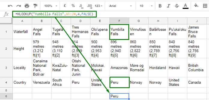
The above HLOOKUP formula searches the text “Yumbilla Falls” in the table range A1:J4 and returns the country name from the fourth row.
How can an HLOOKUP function in Google Sheets return multiple values?
We can use one or more row indexes in the third parameter of the HLOOKUP function in Google Sheets. To do this, we can use curly brackets to enclose the row indexes that we want to return.
For example, the following formula would return the locality and country for the waterfall named “Yumbilla Falls”:
=ARRAYFORMULA(HLOOKUP("Yumbilla Falls",A1:J4,{3,4},false))The HLOOKUP function cannot return multiple values on its own, so you need to use the ARRAYFORMULA function to support it.
Here is a related tutorial: How to return an entire column using the HLOOKUP function in Google Sheets.
Don’t be confused if you see the HSTACK or VSTACK functions within the third parameter of the HLOOKUP function in Google Sheets. They can be used to replace curly braces. For example, you can replace {3,4} with HSTACK(3,4) and {3;4} with VSTACK(3,4).
Horizontal Lookup in a Sorted Range
In Google Sheets, we have interview appointment times in the range B1:F1 and candidate names in the range B2:F2. How do we use the HLOOKUP function to search for a time to find the assigned candidate’s name?
Example:
=HLOOKUP(D6,B1:F2,2,TRUE)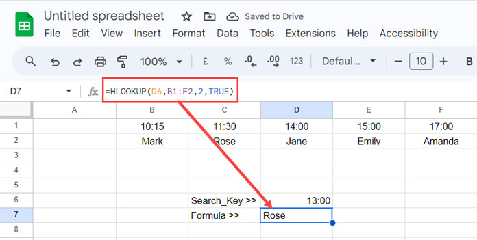
The search key is in cell D6, which is 13:00. Since it is not available in the first row, the formula matches the next smallest time less than the search time, which is 11:30.
We have used TRUE as the last parameter in the formula because the data is sorted. This tells the formula to match the next smallest value that is less than or equal to the search_key, if an exact match is not available.
We can use FALSE in sorted as well as unsorted data. However, if we use FALSE and there is no exact match to the search key, the formula will return the #N/A error.
If the search key in D6 is 15:00, the result would be “Emily”, no matter if you specified FALSE or TRUE as the last parameter in the HLOOKUP function. This is because the value 15:00 is an exact match for the value in cell B5.
Wildcards in HLOOKUP Function in Google Sheets
Wildcards are special characters that can be used in the HLOOKUP function in Google Sheets to match any number of characters or a single character.
One important point that you may not know about using wildcards in HLOOKUP is that you must specify the last parameter, i.e., is_sorted to FALSE.
That being said, the HLOOKUP function supports the following two wildcards: an asterisk (*) and a question mark (?).
Use an asterisk (*) for matching any number of characters and a question mark (?) for matching any single character.
With the following two examples, you can understand how wildcards are used in the HLOOKUP function in Google Sheets.
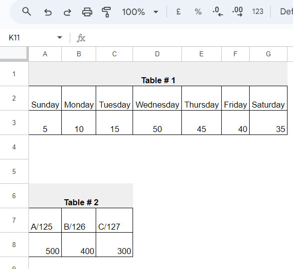
The following HLOOKUP formula in Table #1 will return 50 from the second row.
=HLOOKUP("Wed*",A2:G3,2,FALSE)Do you know why I used the asterisk wildcard in this HLOOKUP?
I used it because I am unsure whether the first row contains day abbreviations (“Wed”) or day full names (“Wednesday”).
The asterisk (*) wildcard matches any number of characters, so in this case, it will match any cell in the first row of the range A2:G3 that starts with the letters “Wed”.
The second HLOOKUP formula in Table #2 will return 400.
=HLOOKUP("B?126",A7:C8,2,FALSE)I used the question mark (?) wildcard in this HLOOKUP formula because I am unsure about the delimiter used in the cell values.
The question mark wildcard matches any single character, so in this case, it will match any cell in the range A7:C8 that starts with the letter “B”, followed by any single character, and then the number “126”.
Note: We can use multiple wildcard characters within a search_key.
How to Clean Up Error Values in HLOOKUP Function in Google Sheets
Some of the most common errors that HLOOKUP returns are as follows:
REF!
HLOOKUP out-of-bounds range: Check whether the index number is correct. In a 2-row range, if you specify any number greater than 2, this error will occur.
The reference does not exist: Check if you have accidentally deleted the range used in the HLOOKUP function.
VALUE!
An array value could not be found: This most likely happens when you use multiple search_keys and forget to use ARRAYFORMULA.
The #VALUE error may also happen when you specify 0 in the index.
N/A
Did not find value 'B?126' in HLOOKUP evaluation: The search_key is not found.
You can wrap the HLOOKUP function in Google Sheets with the IFERROR function to remove those errors. However, I do not recommend doing this, as it will eliminate your chances of troubleshooting the problem.
Instead, you can use the IFNA function. This function will remove only #N/A errors, so you can still troubleshoot the other errors.
Conclusion
I hope you found this step-by-step guide to the HLOOKUP function helpful. If you have any questions or comments, please feel free to post them below.
Here are some related resources for further development in the HLOOKUP function.


