The Vlookup and Hlookup combination can do wonder in Google Sheets. I have seen users using a helper row to get this Vlookup and Hlookup Combination in Google Sheets to work. But I can show you how to use this combination without any helper row or column in Google Sheets.

Clueless, right?

I am talking about two-dimensional lookup in Google Sheets. In this lookup, the Vlookup will do the search across the first column for the provided key and the hlookup will do the search across the first row for another key. Then the formula would return the intersection value.

First, let me clarify the concept about the use of Vlookup and Hlookup together. See how a Vlookup and Hlookup combination in Google Sheets work.

You May Like: Lookup, Vlookup, and Hlookup Differences in Google Sheets

The Purpose of Vlookup and Hlookup Combination In Google Sheets

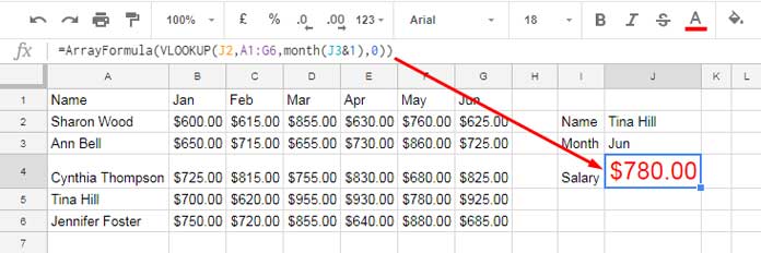
In this example, I have the employee names in Column A and their monthly allowances in other Columns.

I want to find the monthly allowance of a particular employee in a particular month.

Two-way Lookup in Google Sheets Using the Vlookup and Hlookup Combination

First I will explain to you how to do that. Hope you may already know the use of Vlookup.

Formula 1

=VLOOKUP(J2,A2:G6,4,0)

Formula 2

=VLOOKUP("Tina Hill",A2:G6,4,0)

You can use any of the above Vlookup formulas to find the allowance of the employee “Tina Hill” in “Mar”.

In these formulas, the #4 is the column index number of “Mar”.

Unlike Data Base functions like DSUM, we can’t use a field label corresponding to the column name to represent the column. I mean you can’t use “Mar” instead of 4 in Vlookup.

Instead of the column Index 4, we can use an Hlookup inside Vlookup to search and return the column index number corresponding to “Mar”.

Vlookup Syntax:

VLOOKUP(search_key, range, index, [is_sorted])

Vlookup and Hlookup Combination Formula Syntax:

VLOOKUP(search_key, range, HLOOKUP, [is_sorted])

Here is that two-way lookup formula (Vlookup and Hlookup combination formula)

=ArrayFormula(VLOOKUP(J2,A1:G6,hlookup(J3,{A1:G1;column(A1:G1)},2,0),0))

The Hlookup in this formula returns the column Index based on the column name/field label in J3.

Currently, it returns 4 as the field label in J3 is “Mar” which is in the fourth column.

You May Like: Column Heading | Column Label | Column Name | Field | Field Label

Below I am explaining the Hlookup part of the formula.

Hlookup Syntax:

HLOOKUP(search_key, range, index, [is_sorted])

In my above Hlookup formula, the search key is the “Mar” in cell J3. The range is as below.

{A1:G1;column(A1:G1)}

To test this “range” just use it with the ArrayFormula as below.

=ArrayFormula({A1:G1;column(A1:G1)})

Here is the result. It has the field labels in the first row as it is and the second row contains the column numbers. The function Column returns these numbers.

The above Hlookup formula searches across the first row for the key “Mar” in this range and returns the value from the second row, i.e. 4.

See the column Index in Hlookup, i.e. 2 (second row).

This way you can use the Vlookup and Hlookup Combination in Google Sheets.

Two-Way Lookup in Google Sheets – Using Vlookup and Match

Here is an easier solution to the above using Vlookup and Match.

=ArrayFormula(VLOOKUP(J2,A1:G6,MATCH(J3,A1:G1,0),0))

Actually, this tutorial is about the combined use of Vlookup and Hlookup in Google Sheets. Still, I am introducing you to this new combo as this is easy to understand and use.

Here the MATCH just replaces the Hlookup. The match function searches across the first row for the key in J3 and returns the relative position of the key.

Two-Way Lookup Additional Tip

The formula that I am going to provide you below won’t work in all cases.

If your column labels are the month names as above, there is a shorter solution using the Date function. Here is that formula.

=ArrayFormula(VLOOKUP(J2,A1:G6,month(J3&1),0))

Here the Index number is replaced by the Month function. This formula is only applicable to the columns that contain the month names as column names/field labels.

How this Month function returns the column index? Actually, it returns the month number from month name.

Must Read: Formula to Convert Month Name in Text to Month Number in Google Sheets

You have now three different formulas to do a two-way lookup in Google Sheets.

Hope you have enjoyed the stay!