If you want to split a column into multiple columns in Google Sheets, the most effective and modern method is to use the WRAPROWS function. An alternative is using HLOOKUP, which, while older and slightly more complex, allows for advanced control like extracting every nth row.
In this tutorial, I’ll show you two ways to split a single column into multiple columns in Google Sheets, along with real-life use cases, formulas, and explanations.
Why Split a Column into Multiple Columns?
Here are a few practical scenarios where this method is useful:
1. Compact Presentation of Long Lists
Turn a long vertical list into a neater, multi-column layout for better readability and balance.
2. Preparing Labels or Tags for Export
When printing badges, mailing labels, or ID cards, arranging items into multiple columns helps you fit more on a single page.
3. Organizing Related Data
When your data is more readable in a grid format than a long list — like months, names, or scores — this approach improves layout clarity.
Method 1: Split a Column into Multiple Columns Using WRAPROWS
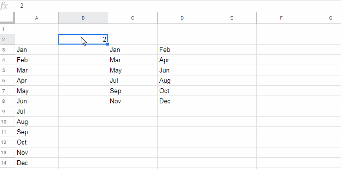
Let’s say you have month names listed from Jan to Dec in the range A3:A14.
In cell B2, enter the number of columns you want — for example, 3.
Then enter the following formula:
=IFNA(WRAPROWS(A3:A14, B2))This will divide the list into rows of three values each, effectively splitting your single column into multiple columns.
Make It Dynamic with an Open Range
If your data is growing over time, use an open-ended range:
=IFNA(WRAPROWS(A3:A, B2))To exclude blank cells, wrap the input with TOCOL:
=IFNA(WRAPROWS(TOCOL(A3:A, 3), B2))This is currently the easiest and cleanest way to split a column into multiple columns in Google Sheets using dynamic arrays.
Method 2: Split a Column into Multiple Columns Using HLOOKUP
HLOOKUP allows more flexibility — particularly when you want to extract values from every nth row instead of sequentially.
Here’s an example:
=ArrayFormula(IFERROR(
   HLOOKUP("title",
      VSTACK("title", A3:A14),
      SEQUENCE(ROUNDUP(ROWS(A3:A14)/B2), B2, 2, 1),
      FALSE
   )
))
Explanation:
- “title” is a dummy search key.
VSTACK("title", A3:A14)adds a fake header to makeHLOOKUPfunctional.SEQUENCE(...)generates the row indexes for values to be returned, skipping the dummy header.
Example: Extract Every 2nd Row (1st, 3rd, 5th…)
Modify the final number in the sequence to 2:
SEQUENCE(ROUNDUP(ROWS(A3:A14)/B2), B2, 2, 2)This way, HLOOKUP can help you create a patterned extraction — something WRAPROWS doesn’t offer directly.
Formula Recap
| Purpose | Formula Example |
| Basic Split into Columns | =IFNA(WRAPROWS(A3:A14, B2)) |
| Dynamic Split with Open Range | =IFNA(WRAPROWS(A3:A, B2)) |
| Exclude Empty Rows | =IFNA(WRAPROWS(TOCOL(A3:A, 3), B2)) |
| Advanced nth Row Split with HLOOKUP | =ArrayFormula(IFERROR(HLOOKUP(...))) |


FYI… This has been provided for by the standard sheets functions…
WRAPROWS and WRAPCOLS
Ie. Using your example, to split into 4 columns you simply use…
=Wrapcols(a3:a14,4)Hi, GF,
Thanks for your comment. I know there are better ways.
I am working in the background to update my 1000+ Google Sheets tutorials. The new functions and Lambda forced me to do it.
I’ll update this post also sooner or later.
It is great! Is there any way to carry over the URLs/rich text value as well?
This formula seems to carry over only the text.
Hi, James,
I think the formula does that. You can try the second method (Hlookup) also.
You can find that URL at the end part of the above tutorial.
Hi! Thanks for all of this! I was wondering if you could think of a way to have them organized in order by column rather than row? So instead of:
Jan | Feb | Mar
Apr | May | Jun
Jul | Aug | Sep
It would be:
Jan | Apr | Jul
Feb | May | Aug
Mar | Jun | Sep
Thanks so much!!!!
Hi, Lee,
The below tutorial may help.
How to Move Each Set of Rows to Columns in Google Sheets
There are two formulas. I recommend option # 2, which is dynamic.
This is amazing! I was hoping there was some built-in function in Sheets to do this and I would not have expected doing this would be so complicated. Your solution saved my day – I don’t think I ever would have figured this out on my own.
I find your site so clear and helpful – I think half of everything I know about using Google Sheets I’ve learned here. Thanks for providing such an excellent resource.
Hi, AS,
Thanks for your feedback! Keep visiting.
Brilliant! Just what I needed.