How to Return an Entire Column in HLOOKUP in Google Sheets

In your horizontal dataset, you might want to use HLOOKUP to return an entire column’s contents. Is this possible? Yes! It’s possible in Google Sheets. See how to return an entire column in HLOOKUP in Google Sheets.

Table of Contents

Introduction

Spreadsheet users typically prefer column-wise (vertical) data formatting because it’s easier to handle, and most Google Sheets functions work better with vertical datasets.

However, you may encounter data arranged horizontally—possibly imported from another source or collected through submissions in Google Forms. In such cases, if you need to look up a value, HLOOKUP (horizontal lookup) can be your go-to function.

As mentioned earlier, the HLOOKUP function can return an entire column from a horizontally arranged dataset. Let’s see how with an example.

Note: While LOOKUP and XLOOKUP can also perform similar tasks, LOOKUP requires sorted data, and XLOOKUP is feature-rich with more options.

Sample Data and the Problem

Here’s our sample data in A1:F4:

Waterfall	Angel Falls	Tugela Falls	Niagara Falls	Victoria Falls	Iguazu Falls
Height (m)	979	948	51	108	82
Locality	Bolívar	KwaZulu-Natal	Ontario/New York	Livingstone	Misiones
Country	Venezuela	South Africa	Canada/USA	Zambia/Zimbabwe	Argentina/Brazil

Problem: In this dataset:

The first row contains the names of waterfalls.
Subsequent rows contain their respective Height, Locality, and Country.

We need to look up a waterfall by name (e.g., “Angel Falls”) and return all its details: Height, Locality, and Country.

Example: Returning an Entire Column with HLOOKUP

To retrieve the Country for “Angel Falls,” you would use the following formula:

=HLOOKUP("Angel Falls", A1:F4, 4, FALSE)

This formula looks for “Angel Falls” in the first row (A1:F1), and returns the value from the 4th row of the corresponding column (B4), which is “Venezuela”.

But what if you want to return the entire column (B1:B4)? Here’s how you can do it:

=ArrayFormula(HLOOKUP("Angel Falls", A1:F4, SEQUENCE(ROWS(A1:F4)), FALSE))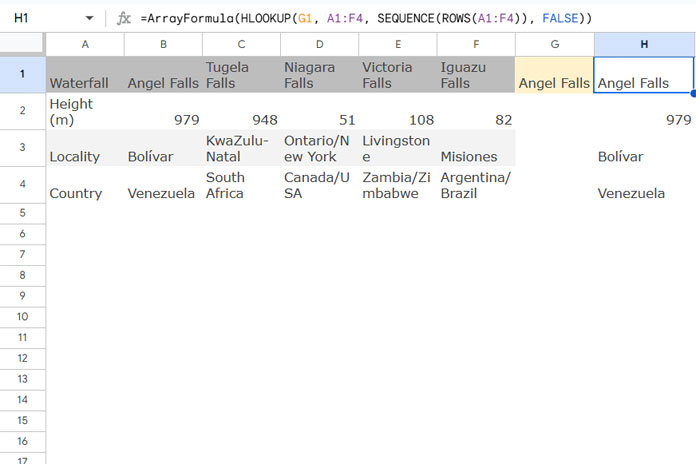

Example of Returning an Entire Column Using HLOOKUP in Google Sheets

You can also use an open range (e.g., A1:F) in the formula for dynamic datasets.

Explanation:

ARRAYFORMULA: Ensures the formula processes multiple values at once.
SEQUENCE(ROWS(A1:F4)): Generates a sequence of index numbers from 1 to the number of rows in the range (1, 2, 3, 4).
HLOOKUP: Uses these sequence numbers to return values from all rows of the column where “Angel Falls” is found.

Return an Entire Column in HLOOKUP While Excluding the Header Row

By default, the HLOOKUP function searches for the key in the first row of the range. If you want to exclude this header row from the results, modify the SEQUENCE function to start from 2 instead of 1:

SEQUENCE(ROWS(A1:F4)-1, 1, 2)

This adjustment ensures the sequence starts at 2 and generates index numbers for rows below the header.

Updated formula:

=ArrayFormula(HLOOKUP("Angel Falls", A1:F4, SEQUENCE(ROWS(A1:F4)-1, 1, 2), FALSE))

How It Works:

ROWS(A1:F4)-1: Reduces the total row count by 1 to exclude the header row.
SEQUENCE(…, 1, 2): Starts the sequence from 2, targeting rows below the header.