The LOOKUP function requires a sorted range to work correctly. If the data is not sorted, use the SORT function in combination with it.
We will use a minimal sample dataset to help you clearly understand all aspects of using the LOOKUP function in Google Sheets.
Syntax
The syntax is as follows:
LOOKUP(search_key, search_range | search_result_array, [result_range])You can use LOOKUP with either two arguments or three arguments:
Two Arguments: search_key and search_result_array
In this method:
- The data must be sorted in ascending order.
- It looks up vertically (top to bottom in the first column) when the number of rows is greater than or equal to the number of columns in the
search_result_array; otherwise, it looks up horizontally (left to right in the first row). - If the search key is not found in the
search_result_array, the formula will look up the largest value in the range that is less than the search key. - It will return the result from the last column (in vertical lookup) or the last row (in horizontal lookup) in the provided range.
- When there are duplicates of search keys, the last occurrence of the search key will be considered.
Three Arguments: search_key, search_range, and result_range (similar to what you may see in XLOOKUP)
All the points above are applicable here as well, except the second point, which does not apply since we are using two individual arrays.
Using the LOOKUP Function with Two Arguments: Examples
Let’s use minimalistic data for this test to help you better understand the function.
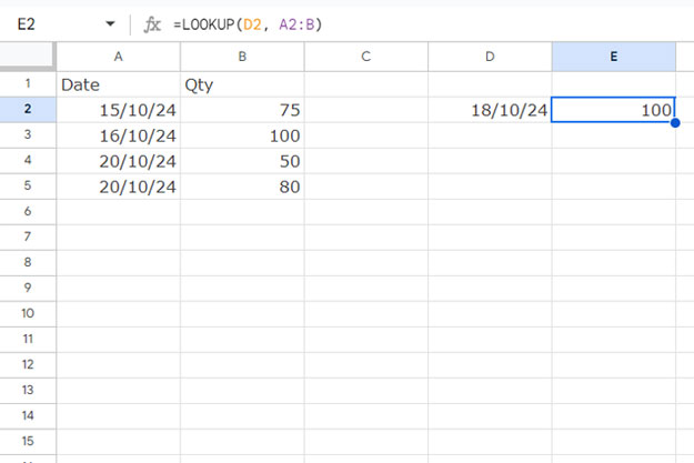
The sample data is in range A1:B, where column A contains delivery dates and column B contains quantities delivered.
Enter 18/10/2024 in cell D2 and the following formula in E2:
=LOOKUP(D2, A:B)This will return 100 since the date 18/10/2024 is not available in the first column. The next lowest available date is 16/10/2024, so the formula returns 100 from the same row in the last column.
Change the date in D2 to 20/10/2024. The formula returns 80 because the search key occurs twice, and it considers the last occurrence.
If the data aligns horizontally in the range 1:2, you can use the following formula to look up the search key in cell B5 in the first row and return the value from the last row, which is the second row.
=LOOKUP(B5, 1:2)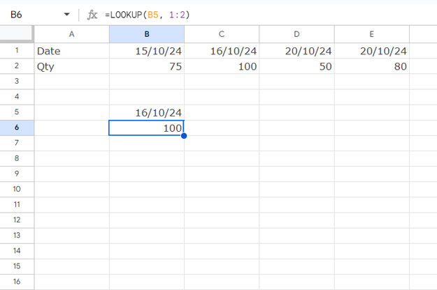
Using the LOOKUP Function with Three Arguments: Examples
As mentioned earlier, the LOOKUP function with three arguments strictly follows all the features of the two-argument formulas described above.
Let’s start with the LOOKUP function in vertical data:
=LOOKUP(D2, A:A, B:B)This will return 100 when the search key is 18/10/24 in cell D2 and 80 when the search key is 20/10/24.
For horizontal data, try these formulas:
=LOOKUP(B5, 1:1, 2:2) // returns 100 when B5 is 18/10/24, 80 when B5 is 20/10/24
Compared to the two-argument LOOKUP, the three-argument version offers the flexibility to return results from any specified column (in vertical lookup) or row (in horizontal lookup).
Combining SORT and LOOKUP Functions
The best way to use LOOKUP is to work with sorted data. However, if you don’t want to alter the original data but still perform a lookup, you can use functions like VLOOKUP, XLOOKUP, or HLOOKUP. Alternatively, you can use the SORT function in combination with LOOKUP.
Here is the data in A1:B:
| Item | Qty |
| Orange | 7 |
| Apple | 3 |
| Orange | 6 |
| Mango | 2 |
| Banana | 1 |
Here’s how to correctly apply the LOOKUP function to unsorted data in Google Sheets:
Two-Argument LOOKUP Formula:
=LOOKUP("Orange", SORT(A2:B, 1, 1)) // returns 6In this formula, the search_result_array is sorted within LOOKUP by the first column in ascending order.
Three-Argument LOOKUP Formula:
=LOOKUP("Orange", SORT(A2:A, 1, 1), SORT(B2:B, A2:A, 1)) // returns 6Here:
- The
search_rangeisSORT(A2:A, 1, TRUE), which sorts the items in column A in ascending order. - The
result_rangeisSORT(B2:B, A2:A, TRUE), which sorts column B based on the values in column A.
Resources
- How to Get LOOKUP Results from a Dynamic Column in Google Sheets
- How to Lookup Latest Dates in Google Sheets
- How to Find the Last Matching Value in Google Sheets
- How to Perform Two-way Lookup Using Vlookup in Google Sheets
- Two-way Lookup and Return Multiple Columns in Google Sheets
- Two-Column Output in a Two-Way Lookup in Google Sheets
- Three-way Lookup in Google Sheets [Array and Non-Array Formulas]
- Find and look for Target Sum Reached Row in a Column in Google Sheets
- How to Lookup First and Last Values in a Row in Google Sheets
- 4 Formulas to Last Row Lookup and Array Result in Google Sheets
- How to Get the Cell Address of a Lookup Value in Google Sheets
- Conditionally Lookup Dates in Start-End Ranges in Google Sheets


