Do you need to retrieve a value from a specific column in Google Sheets based on a date or other criteria? Using the LOOKUP function, you can search for a value in one column and return the corresponding result from a dynamic column in a range.

For example, you can search today’s date in column A and return the price of apples from a column range containing mango, apple, banana, and orange prices. This guide will walk you through step-by-step instructions to set up a dynamic column lookup in Google Sheets.

Sample Data

Here’s the example dataset we will use for this tutorial:

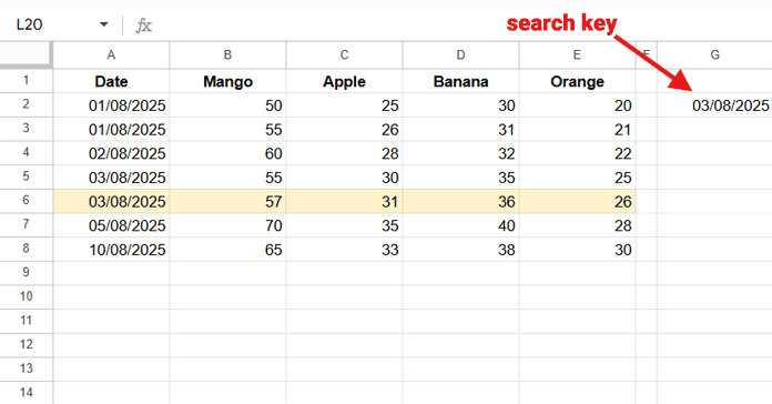
We will use the LOOKUP function in this table to find the price of Apple on 03/08/2025 dynamically. Note that for basic LOOKUP to work properly, the data in the first column (Date) must be sorted in ascending order.

Overview of the LOOKUP Function in Google Sheets

The LOOKUP function can be used in two ways when the data range is sorted:

1. Simple LOOKUP across a range

=LOOKUP(G2, A2:E) // returns 26

• Matches the last occurrence of the search key in A2:A.
• Returns the value from the last column of the range (E in this example).

2. LOOKUP with a specific return column

=LOOKUP(G2, A2:A, C2:C) // returns 31

• Matches the last occurrence in column A.
• Returns the corresponding value from C2:C (Apple column in this example).

Limitation: This method works only when the return column is fixed. If you want to lookup the column dynamically, you need a different approach.

Note: The LOOKUP function works in a sorted range. It:

• Matches the value that exactly equals the search key, if it exists.
• If there is no exact match, it matches the largest key that is smaller than the search key.
• When the search key occurs multiple times, LOOKUP matches the last occurrence of that key.

How to LOOKUP a Value from a Dynamic Column in Google Sheets

To lookup a value from a dynamic column, you can use either:

1. FILTER function
2. CHOOSECOLS and XMATCH combination

Using CHOOSECOLS and XMATCH

=CHOOSECOLS(A2:E, XMATCH("Apple", A1:E1))

• XMATCH("Apple", A1:E1) finds the position of the column header “Apple”.
• CHOOSECOLS(A2:E, …) selects that column from the range.

Using FILTER (Preferred)

=FILTER(A2:E, A1:E1="Apple")

• Directly filters the range A2:E to include only the column with header “Apple”.
• More straightforward and easier to understand.

Combining with LOOKUP

=LOOKUP(G2, A2:A, FILTER(A2:E, A1:E1="Apple"))

• G2 contains the date to search.
• FILTER(A2:E, A1:E1="Apple") dynamically returns the Apple column.
• This formula performs a dynamic column lookup in Google Sheets.

Lookup Dynamic Columns in Unsorted Google Sheets Data

If your data is not sorted, the best approach is using XLOOKUP:

=XLOOKUP(G2, A2:A, FILTER(A2:E, A1:E1="Apple"), , -1, -1)

• Searches for the date in G2 within A2:A.
• Returns the value from the dynamic column returned by FILTER.
• The first -1 ensures the search starts from last to first, which helps when dates are repeated.
• The second -1 sets the match mode to exact match or next smaller value.

Frequently Asked Questions (FAQ)

Q1: What is a dynamic column lookup in Google Sheets?
A dynamic column lookup allows you to search for a value in one column and return a corresponding value from a column that is determined dynamically, instead of being fixed. This is useful when the return column may change based on a header or criteria.

Q2: Can I use LOOKUP for dynamic columns in unsorted data?
No, the standard LOOKUP function requires a sorted range to work correctly. For unsorted data, it’s recommended to use XLOOKUP combined with FILTER or other dynamic formulas to get accurate results, even when dates or search keys are repeated or out of order.

Q3: Should I use FILTER or CHOOSECOLS + XMATCH for dynamic columns?
Both work, but FILTER is simpler and more straightforward for most cases.

Example Sheet

Click the button below to make a copy of the sample Google Sheet and try these formulas yourself.

Copy Sample Sheet

Related Resources

• Dynamic Index Column in VLOOKUP in Google Sheets
• Dynamic Return Column in VLOOKUP IMPORTRANGE in Google Sheets
• Dynamically Change the Search Column in VLOOKUP in Google Sheets
• How to Perform Two-Way Lookup Using VLOOKUP in Google Sheets
• Two-Way Lookup and Return Multiple Columns in Google Sheets
• Two-Way Lookup with XLOOKUP in Google Sheets