How to Find the Last Matching Value in Google Sheets

This tutorial describes how to find the last matching value in Google Sheets using the LOOKUP and XLOOKUP (new) functions. The tips apply to both sorted and unsorted data.

You may find this lookup skill useful in many real-world situations, such as finding the last time the price of an item changed, or the last time a customer made a purchase.

Example of the last matching value:

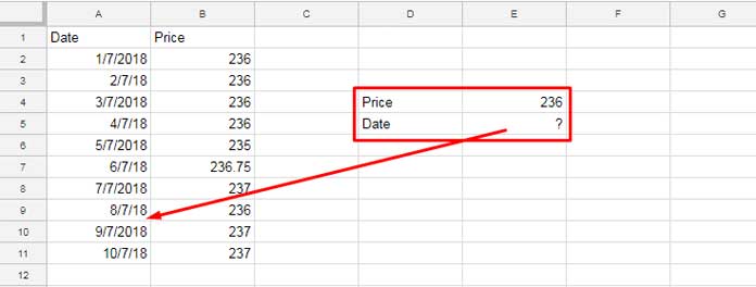
The above list shows the changes in the price of an item over the last 10 days.

I want to search down the “Price” column (column B) for the last appearance of the price 236 and return the corresponding date from column A. This will allow me to understand when the price was changed most recently.

In other words, I want to find the last matching value in Google Sheets. There are two easy solutions using the LOOKUP function, and which one you use depends on how you have arranged your data.

Solution 1 is for unsorted data, and solution 2 is for sorted data. In the above example, the column that contains the price is not sorted. Therefore, we can use solution 1 here.

If you use XLOOKUP, you don’t need to worry about sorting. We will see that in the later part of this tutorial. We will start with LOOKUP.

Before we write the formula, I need to explain some essential LOOKUP tips.

LOOKUP Function: Essential Tips for Google Sheets

The LOOKUP function has an edge over VLOOKUP and HLOOKUP because it can work on both horizontal and vertical datasets, and it can return the last matching value in a lookup.

The LOOKUP function has the following syntax:

LOOKUP(search_key, search_range,result_range)

Example:

=LOOKUP(3, {1,3,3,4}, {"a","b","c","d"})

Result: “c”

That means if the search key is found, it will return the last matching value. Now see what happens when the search key is not present.

=LOOKUP(6, {1,3,3,4}, {"a","b","c","d"})

Result: “d”

Here, the search key 6 is not present in the lookup range. Therefore, the value that is immediately smaller than 6 and present in the lookup range will be considered.

Find the Last Matching Value in Unsorted Data in Google Sheets (Solution 1)

The LOOKUP function is one of the most efficient solutions for finding the last matching value in Google Sheets. XLOOKUP is a newer function that is also very efficient.

I know that the former function only works efficiently with sorted data, but our data is not sorted. However, we can work around this by following two methods.

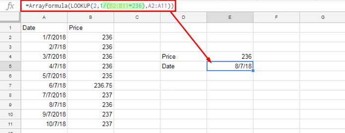
Method 1: By Using 1 and #DIV/0! in Lookup Range

As per our example in Figure 1 above, we want to find the last row where the price 236 is found in the range B2:B11 and return the date from the range A2:A11 from that row.

The following LOOKUP formula has a hardcoded condition.

=ARRAYFORMULA(LOOKUP(2,1/(B2:B11=236),A2:A11))

To use a cell reference for the condition, for example, cell E6, enter the condition value, 236, in cell E4 and use the following LOOKUP formula:

=ARRAYFORMULA(LOOKUP(2,1/(B2:B11=E4),A2:A11))

The result of the formula is 08/07/2018, which is the date when the price 236 was last found in the price column (column B).

See the formula again and pay particular attention to the green highlighted part, which is 1/(B2:B11=236).

Find the Last Matching Value in an Unsorted Range in Google Sheets — Figure 2

In that, the formula B2:B11=236 returns TRUE or FALSE depending on whether the value 236 is found in the range B2:B11. By dividing this formula by 1, we get 1 for TRUE and #DIV/0! for FALSE.

{1;1;1;1;#DIV/0!;#DIV/0!;#DIV/0!;1;#DIV/0!;#DIV/0!}

It’s the lookup range (search_range) in LOOKUP. In my LOOKUP formula, you can see that the search_key is 2. Since this key is not available in the lookup range, the LOOKUP will find the last matching value, i.e. 1 in the 8th row of the lookup range, and return the date from the result range.

=LOOKUP(2, {1;1;1;1;#DIV/0!;#DIV/0!;#DIV/0!;1;#DIV/0!;#DIV/0!}, {"01/07/2018","02/07/2018","03/07/2018","04/07/2018","05/07/2018","06/07/2018","07/07/2018","08/07/2018","09/07/2018","10/07/2018"})

Note: The dates within this explanation formula are based on the default date format in my Sheet.

Method 2: By Virtually Sorting the Lookup Search_Range and Result_Range

Here is another method to find the last matching value in a range in Google Sheets. It’s by virtually sorting the lookup range and the result range.

The formula is:

=IF(MATCH(E4,B2:B11,0),TO_DATE(LOOKUP(E4,SORT(B2:B11),SORT(A2:A11,B2:B11,1))))

Formula Explanation:

The SORT formula sorts the range in ascending order by default. So, the following formula sorts the B2:B11 range in ascending order:

SORT(B2:B11)

Syntax: SORT(range, sort_column, is_ascending, [sort_column2, …], [is_ascending2, …])

We must sort the A2:A11 range according to the B2:B11 range.

To do this, we must specify the sort_column range and is_ascending in the formula. This tells the formula to sort the range A2:A11 by the values in the B2:B11 range in ascending order.

SORT(A2:A11,B2:B11,1)

The rest of the formula parts are optional. They are TO_DATE and IF + MATCH. The former formats the result, which is usually a date value, to a proper date, whereas the latter helps to execute the formula if there is an exact match of the search key available in the lookup range.

Find the Last Matching Value in Sorted Data in Google Sheets (Solution 2)

You have learned the more complicated part first. So here, things are simpler.

Here, B2:B11, the lookup range, is sorted. So we can use the following LOOKUP formula to find the last matching value in a sorted range in Google Sheets.

=IF(MATCH(E4,B2:B11,0),LOOKUP(E4,B2:B11,A2:A11))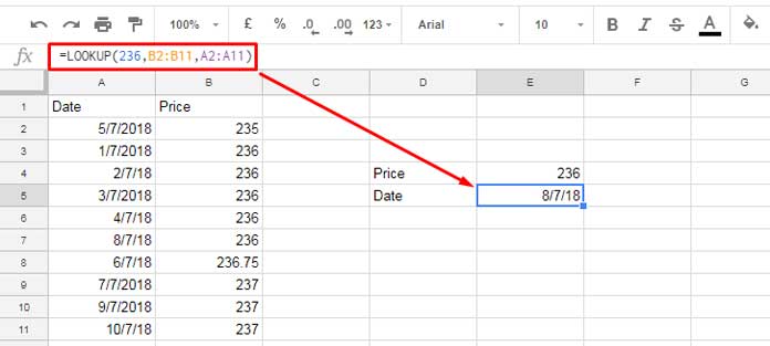

I have already explained the role of IF + MATCH in the earlier example. It is to execute the LOOKUP formula if the search key is present in the search range.

XLOOKUP: The New Google Sheets Function to Find the Last Matching Value

XLOOKUP was not available when I first wrote this tutorial. So, I used the LOOKUP function to find the last matching value.

All of the above formulas will work well. However, XLOOKUP is much simpler than all of them.

Syntax:

XLOOKUP(search_key, lookup_range, result_range, [missing_value], [match_mode], [search_mode])

It does not have any issues in finding the last matching value in a sorted or unsorted range. You can use the following formula regardless of whether your data is sorted or unsorted.

=XLOOKUP(E4,B2:B11,A2:A11,"Missing",0,-1)

In this formula, you can replace the word “Missing” with any custom text.

31 COMMENTS

David Laks August 31, 2023 At 3:57 am

Hello!

I notice that the sorted formula returns the next closest value if the lookup reference does not exist. This can be unrelated to the value I am looking for. I am searching for an SKU (part number) and the first date it was sold within sorted data. If the SKU happens to never have been sold and is not on the list, then the formula returns the first sale date of the next closest SKU. How can I prevent this?

- Prashanth August 31, 2023 At 6:53 pm
  
  Hi David Laks,
  
  We can use XLOOKUP. I’ll update the post as soon as possible.
  
  Thanks.
  
Nagarjuna AS July 17, 2021 At 9:51 am

This helps a lot within a sheet, but how about between google sheets, how can we get the latest value in the column between google sheets.

- Prashanth July 17, 2021 At 9:57 am
  
  Hi, Nagarjuna AS,
  
  We can use Query Importrange. But that depends on your data.
  
  If you share more details or a sample sheet, I would be able to suggest one formula.
  
Dan May 26, 2021 At 4:12 am

Hello, I’m using a google form to collect data and I want my output to be several cells of the last entry from a given name. I’m having trouble combining the functions of locating the latest entry for a name and then extracting the specific cell based on that search/sort.

Any help is appreciated,
Thanks!

- Prashanth May 26, 2021 At 8:33 am
  
  Hi, Dan,
  
  Thanks for sharing your sheet. You require SORTN to get the latest entry from each name from your form submission.
  
  This formula will do that for you (only try it in a new tab in your sheet).
  
  =sortn(sort(Data!A2:G,3,1,1,0),9^9,2,3,1)
  
  You want just 4 columns in the output. So Let’s Query the above result.
  
  =query(sortn(sort(Data!A2:G,3,1,1,0),9^9,2,3,1), "Select Col3,Col5,Col6,Col7")
  
  Now let’s use the above output in a Vlookup to assign it to correct names.
  
  Go to the “Output” tab, and remove all the existing formulas. Insert the below formula in E3.
  
  =ArrayFormula(IFNA(Vlookup(B3:B, query(sortn(sort(Data!A2:G,3,1,1,0),9^9,2,3,1), "Select Col3,Col5,Col6,Col7"),{2,3,4},0)))
  
Zyshan March 22, 2021 At 12:56 am

Hello Prashanth,

I am sharing my sheet with you regarding the information you have shared.

- Prashanth March 22, 2021 At 9:34 am
  
  Hi, Zyshan,
  
  The problem is that you have blank values in the result column. So you get a blank sometimes.
  
  Unlike in the tutorial, in your case, you want to search a text (its last occurrence) in column E and get the corresponding number from column F. If the number column contains blank, the formula will return that.
  
  To avoid that, Filter the columns to exclude blanks.
  
  I have already inserted the formula and some notes in your Sheet.
  
  - Zyshan March 22, 2021 At 10:17 pm
    
    Thank you so much for always being there for the help.
    
    Great soul
    
seth June 28, 2020 At 7:51 pm

I have a job board for work. My boss wants a dashboard now of a list of the dates a job was done last…. Will this formula somehow work if it’s not just 2 columns but instead 365 and it’s just looking for the last time X job was used in relation to the date? Or am I totally off track here?

- Prashanth June 29, 2020 At 9:23 am
  
  Hi, Seth,
  
  The formula has no relation to the date. Instead, it considers the last position in the order. The formula would work with any number of columns. I have noted you want a list of dates. So I’m not fully clear about your requirements.
  
  I could help you if you can fulfill the following:
  
  1. Sample Sheet with some mockup data.
  2. The result (dashboard) you want from the mockup data in the same file.
  
  If you share the file, I would be able to make a copy and try my formula. Your shared sheet here won’t be published.
  
Simon Larsen April 21, 2020 At 2:06 pm

Hi,

Please help with a formula to give the last value (score) from timestamp (Google Forms submission)

As submissions are from timestamps, the names and scores are not sorted. How can scores be updated on the Data tab with the last value?

Thanks for this page, you helped me with some formulas.

- Prashanth April 22, 2020 At 2:58 pm
  
  Hi, Simon Larse,
  
  I have checked your sheet and entered my following formula in Data!B2.
  
  =ArrayFormula(IFNA(vlookup(A2:A;sort({'Form Submission'!B2:C\regexreplace('Form Submission'!A2:A;":";".")};3;0;1;0);2;0)))
  
  Explanation:
  
  Your sample data has three columns – Timestamp (Column A), Name (Column B) and Score (Column C) – and the tab name is ‘Form Submission’.
  
  Actually in column A, the values look like timestamp, but it’s in the wrong format. As per your locale, timestamp must be 08/04/2020 23.19.40 not like 08/04/2020 23:19:40.
  
  Using Regexreplace I have corrected that timestamp and sorted the output in descending order (date column). Also, the column order re-arranged like Name (Column A), Score (Column B), Timestamp (Column C).
  
  sort({'Form Submission'!B2:C\regexreplace('Form Submission'!A2:A;":";".")};3;0;1;0)
  
  The search keys are in Data!A2:A that are the names. The above is the range. Using Vlookup, I have searched the keys in A2:A in the above formatted ‘range’ and extracted the score from the second column.
  
  Since the data is sorted in descending order, the latest values are in the top rows. So Vlookup will return the correct (latest) scores.
  
Nathan February 1, 2020 At 8:31 pm

Thank you so much, Prashanth!

I added a column, but also put up another sheet with something that is closer to what I’m trying to do.

Ultimately I want to flag the customer (in another sheet) when they are past due. I’ve managed to flag the invoice item (see the new tab).

It would be useful to see how many payments are remaining and when they are due. But mostly I need to flag them so when they show up, we know. Hope that makes sense.

- Kevin Canadian March 28, 2020 At 2:43 am
  
  Sounds like you might want to have an Aging column where you’d evaluate based on =NOW().
  
  So something like:
  
  =INT(NOW()-(LOOKUP_lastvalue_as_shown_above))
  
  Then use conditional formatting to flag values >30.
  
  Hope this helps!
  
Nathan February 1, 2020 At 12:40 am

I managed to implement what you describe …somewhat. But I’m unable to get it in the shape I need. If you are able, I’d really appreciate your thoughts. I’m probably going about this all wrong.

I’m trying to track (here and on another sheet) if payments have been made, how much is owed BUT…

…most importantly if the payment is due.

I know when the invoice comes in: how much, how many payments, and when the payments are due.

I need to be able to tell the difference between an outstanding balance and an outstanding balance with an aging > 30 days.

This is why I thought I needed to use the formula we are discussing. Have a look at this sheet if you would. I’ve managed to calculate a running tab as payments (+) are applied against invoices (-). I just can’t seem to connect the dots.

- Prashanth February 1, 2020 At 9:01 am
  
  Hi, Nathan,
  
  I’ve checked the sheet. Please just insert one more tab in that file and enter your required output (manually). So that I can work on it.
  
Nathan January 31, 2020 At 5:38 am

Would it be possible to couch this formula into an arrayFormula allowing it to populate an entire column without the need to drag the contents down the column?

This would be used to lookup the last payment and payment date on record in a balance sheet where each row is a payment generated by a user.

I want to track repeating payments and flag them when they are overdue.

- Prashanth January 31, 2020 At 8:58 am
  
  Hi, Nathan,
  
  I assume the data must contain a date column or a sequential number column since it’s related to payments.
  
  If so, there is no need to use Lookup. We can extract the rows containing last payments using a SORT and SORTN combination formula.
  
  You may please check this tutorial – Find the Last Entry of Each Item from Date in Google Sheets.
  
  If this doesn’t solve the mentioned problem, you can share a copy of your sheet after replacing original data with sample data.
  
Leon January 7, 2020 At 8:18 pm

Great formula man, thanks for sharing.

However… 😀 I’m having an issue with for some reason and I was hoping you could lend a hand?

My main goal is to simply look for the last mileage entry for vehicles from the previous month.

To do this so far I have used Importrange to get the previous spread sheet’s values into the current month. I want to then use your formula to get the last entry based on the vehicle reg number. But for some reason I keep ending up with the N/A error:

Did not find value ‘2’ in LOOKUP evaluation.

Strange thing is, the correct mileage is displayed in the formula helper window @ the top left. But as soon as I hit enter, I get the error.

ALSO, I’ve tried this a day before and it actually was working, yet it was taking forever to actually do the calculations.

Any thoughts or suggestions? I would really appreciate it.

Kind regards

- Prashanth January 8, 2020 At 9:40 am
  
  I am unable to say the reason, as there may be many, for the error without seeing your data.
  
  What you can do is;
  
  I have updated my post with a new ‘Method 2’ formula (under a new subtitle). Try that too. Again, having problem? Consider making a demo sheet and share.
  
Tanveer Singh December 5, 2019 At 3:36 pm

Hi Prashanth,

Thank you for sharing your knowledge with the world.

Could you please suggest to me how to use a lookup formula to derive relative cell value from another google spreadsheet for the last matching value.

Thanks again!!

Peter November 16, 2019 At 8:24 pm

Hi, Prashanth,

What if I want to find the first matching value, what formula would I use?

Thank you a lot!!

- Kevin Canadian March 28, 2020 At 2:35 am
  
  You can just use VLOOKUP or HLOOKUP for that.
  
Michael D October 3, 2019 At 4:24 am

Hi Prashanth,

Thanks very much for this, it has been very useful. I have been applying your formula and it has been working great, however, I have run into an issue that I was hoping you could help me with.

I have a sheet that is populated via form entries, the form collects a user name, a value, along with time-stamping them and saves to a sheet, then I have been using your formula to calculate the latest entry for a list of users- I’ve been doing this with:

=ArrayFormula(IFERROR(LOOKUP(2,1/ (Submissions!$A$2:$A$101=$A2), Submissions!$B$2:$B$101)))

where A2 is the name of the person I’m trying to find the latest entry for on the Submission sheet. I then have to drag this formula down to cover every name.

When using forms it always adds data to the first blank row. As so my other calculations use ArrayFormulas for the whole column and are based off IF is blank then do nothing, otherwise, FORMULA).

The problem is even when using the IFERROR clause so the cells appear blank, the form still adds to the first row where that doesn’t have the last entry calculation formula applied to it. I’ve been trying something like the below to no avail:

=ArrayFormula(IFERROR(LOOKUP(2, 1/(Submissions!$A$2:$A$101=$A$2:$A),Submissions!$B$2:$B$101)))

I’m looking for a way I can apply the formula to the whole list of users (which can change) without having to copy the formula down. Any thought’s on this? Any help would be much appreciated. Thank you.

- Prashanth October 3, 2019 At 10:26 am
  
  Hi, Michael D,
  
  Since you have Timestamp recorded, we can try a different formula to return an array result.
  
  What about sharing a replica of your sheet? If not interested try this method.
  
  Sample Data on the “Submissions” tab.
  
  Timestamp|Name|Marks
  03/10/2019 10:26:36|Test Name 1|98
  03/10/2019 11:26:36|Test Name 2|96
  03/10/2019 12:20:30|Test Name 1|87
  04/10/2019 10:01:00|Test Name 3|90
  04/10/2019 16:04:14|Test Name 2|91
  05/10/2019 11:45:45|Test Name 2|100
  
  The formula on the “Formula” tab.
  Name|Formula
  Test Name1|*array formula here
  Test Name 2|
  
  *Formula:
  
  =ArrayFormula(IFNA(vlookup(A2:A, query(sortn(sort(Submissions!A2:C,1,0),9^9,2,2,0), "Select Col2,Col3"),2,0)))
  
  Best,
  
Frances September 12, 2019 At 10:51 am

Do you know how we can find the last matching value if the search query is a letter, not numerical?

For example, in column A I have multiple rows with value of “DE”. In Column B I have a variety of values that match with “DE”. I want to use LOOKUP to find the last row in Column B that has the corresponding value of “DE” in column A.

- Prashanth September 12, 2019 At 2:23 pm
  
  Hi, Frances,
  
  The same tips applicable here.
  
  =ArrayFormula(lookup(2,1/(A2:A="DE"),B2:B))
  
  Best,
  
  - Kevin Canadian March 28, 2020 At 2:32 am
    
    I have a large data set of repeated tests and I’m looking for the last result (the accepted result). You’ve helped me enormously!
    
    I had to tweak it a bit as I too am looking for a text string (ID of unit) in Column A then looking for the result in Column D. I found this worked:
    
    =IFNA(ARRAYFORMULA(LOOKUP(500,1/('TestData'!$A$2:$A=C27), 'TestData'!$D$2:$D)))
    
    I added the IFNA to keep my report page clean (removed #NAs when you drag this down to rows where there is no match yet.. i.e. test hasn’t been done on that unit).
    
    You’ll note the 500 as the search_key … this I found through trial & error since I have hundreds of rows in my data set, I chose an arbitrarily large number to ensure it gives me back the last value in the array result.
    
    Thanks again!
    
Andrew Nelson December 6, 2018 At 8:31 pm

Can this be expanded to have 2 search criteria?

eg, taking the original example, adding a 3rd column for say, store location. 1-6 are York, the Rest are Leeds. I want the last date 236 was sold, In York? (ie A6’s content of 4/7/18) can this be worked?

- Prashanth December 7, 2018 At 2:16 pm
  
  Hi, Andrew,
  
  I think yes. You can tweak the formula as below.
  
  =ArrayFormula(LOOKUP(2,1/(B2:B11&C2:C11="236York"),A2:A11))
  
  Please see how I have combined the criterion and corresponding columns. I’ll try to write a tutorial on this soon.
  
  Cheers!