Finding the last entry of a single item is just child’s play in Google Sheets. Just sort the date column in descending order. The top row will contain the last entry. By saying last entry, I mean the row that contains the latest date.
But what about the last entry of each item or a group of items? In Google Sheets, it’s easy.
Of course, sorting is not a solution. I should say ‘normal’ sorting is not a solution. Do you know why?
Please follow my example. I have hidden the answer below.
Before that, one more thing. Do you know where comes such a requirement? Why does one want to find the last entry of each item based on a date column?
The Purpose of Finding the Last Entry of Each Item
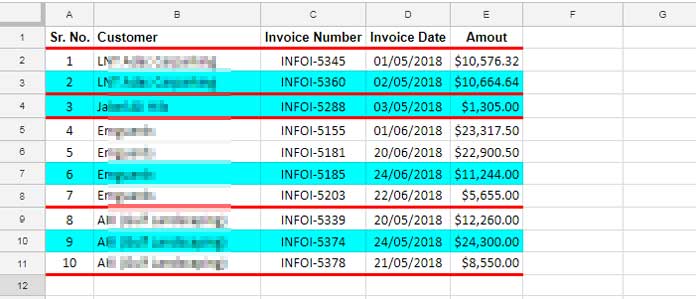
In Accounts, you can follow this method to find the last invoice submitted by each company. The below screenshot is in line with this concept.
If you are in the transport business, in a flash, you can find the halting time of your trucks/busses/rental cars on a specified day.
In HR & ADMIN, you can use it to track the latecomers.
In countless similar scenarios, you can use my formula to find the last entry in each group in Google Sheets.
Steps to Find the Last Entry of Each Item from Date in Google Sheets
Sample Data:

In this example, I have separated each group with red-colored lines.
The cyan highlighted rows are the latest entry in that group. I mean the latest based on the “Invoice Date” column, the fourth column in the range A2:E.
Please go through the dates in each group, and you can understand this.
From this dataset, I want to extract/retrieve the highlighted rows separately. How?
It’s not much complicated as you think. Here is that killer formula.
The Formula to Extract the Last Entry of Items in Google Sheets
Master Formula
=SORTN(SORT(A2:F,4,0,2,1),9^9,2,2,1)I’ve used two Google Sheets functions in this master formula: SORT and SORTN.
Here is how they retrieve the last entry of each item based on the date column.
Formula Explanation and Logic
First, I want the last entry of items at the top of the groups. See this example with one fruit item.
25/05/2018 Apple
26/05/2018 Apple
23/05/2018 Apple
In this, the dates are in column 1, and the text strings “Apple” are in column 2.
If I sort column 1, i.e., the date column, in descending order, the above data will be as below.
26/5/18 Apple
25/5/18 Apple
23/5/18 Apple
It is what the SORT function in the above formula does. Here is that SORT formula part only.
=SORT(A2:E,4,0,2,1)In this formula part, the number 4 is the column index number of the date column in our dataset. The number 0 indicates sorting this column in descending order.
In addition, I’ve sorted column 2 in ascending order as we have multiple text strings (customers in column 2). It helps group them.
As I’ve told you, we only want to retain one item from the group. I mean the top row in each group. The SORTN formula does this part wonderfully. How?
Please scroll back and see my formula that finds the last entry of each item.
Now see this SORTN syntax.
SORTN(range, [n], [display_ties_mode], [sort_column], [is_ascending], [sort_column2, …], [is_ascending2, …])In this syntax of the SORTN function, “range” is the just above-provided SORT formula.
The “n” argument represents the number of rows in the SORTN result.
Since we are unsure about the number of rows after removing each repeated item, I’ve opted to put 9^9, which is an arbitrarily large number.
The display_ties_mode is 2. It removes repeated items. It works based on the “sort_column.”
The “sort_column” must be the column index number of the group column, i.e., 2.
Conclusion
You can find the last entry of each item in Google Sheets in many ways. Among them, the use of the SORT and SORTN combination is a tricky one.
It seems Google Sheets users are yet to widely use this combo.
Related:


Hi Prashanth 😊
I need to pull out every last data for every end of the month in C9, C16, C20. thank you.
Hi, Bahar,
Thanks for the sheet link.
We can’t use the formula mentioned in this tutorial to solve the problem. I’ll come back to you with a new tutorial soon.
Hi, Bahar,
I have inserted the formula into your sheet.
Here you can find the explanation and an alternative formula too.
Return Month End Rows from Daily Data in Google Sheets.