To return month-end rows from daily data in Google Sheets, you can use the FILTER function together with EOMONTH.
If multiple records exist for the same month-end date, the basic formula returns all of them. Depending on your requirements, you can also return only the first or last occurrence for each month-end date by combining FILTER with SORT and SORTN.
This tutorial covers all three approaches.
Why Return Month-End Rows?
Suppose you maintain a daily inventory valuation sheet that records the total inventory value for each day.
Although the data is recorded daily, monthly reports often require only the records dated on the last calendar day of each month. Extracting those month-end rows makes it easier to prepare month-end summaries, compare inventory values across months, or create charts without manually filtering the data.
In this tutorial, the formulas return only the rows whose dates fall on the last day of their respective months. If a month doesn’t contain a record on its final calendar day, no row is returned for that month.
Example: Return Month-End Inventory Valuation Records
The following sample data contains inventory valuation dates in column A and the corresponding inventory values in column B. The first row contains the column headers, so the data range is A2:B.
| Date | Inventory Value |
|---|---|
| 2 Jan 2026 | 145600.00 |
| 18 Jan 2026 | 147100.00 |
| 31 Jan 2026 | 149300.00 |
| 3 Feb 2026 | 148900.00 |
| 28 Feb 2026 | 151200.00 |
| 2 Mar 2026 | 150700.00 |
| 29 Mar 2026 | 152100.00 |
| 31 Mar 2026 | 152900.00 |
Use the following formula to return all rows whose dates are the last calendar day of their respective months:
=FILTER(A2:B, A2:A=EOMONTH(A2:A, 0))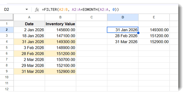
Note: These formulas return only rows whose dates are the actual last calendar day of each month. If a month doesn’t contain a record on its final day, no row is returned. If you instead want the latest available record for each month, see Extract the Last Entry of Each Item by Date in Google Sheets.
The formula compares each date in column A with the last calendar day of its month returned by EOMONTH. It then uses FILTER to return only the rows where the two dates match.
If your data contains multiple records for the same month-end date, the previous formula returns all of them.
To return only the first occurrence for each month-end date, use:
=LET(
  eomData, FILTER(A2:B, A2:A=EOMONTH(A2:A, 0)),
  SORTN(eomData, 9^9, 2, 1, TRUE)
)
FILTER first returns all month-end rows and stores the result in eomData. SORTN then removes duplicate dates while keeping the first occurrence of each date.
To return the last occurrence for each month-end date, first reverse the filtered rows and then apply SORTN.
=LET(
  eomData, FILTER(A2:B, A2:A=EOMONTH(A2:A, 0)),
  fData, SORT(eomData, SEQUENCE(ROWS(eomData)), 0),
  SORTN(fData, 9^9, 2, 1, TRUE)
)
The formula first filters the month-end rows, reverses their order, and finally uses SORTN to remove duplicate month-end dates while keeping what was originally the last occurrence.
FAQs
Can I include the header row?
Yes. You can reference A1:B and A1:A instead of A2:B and A2:A. The header row is automatically excluded because EOMONTH returns an error for the text header, causing FILTER to ignore that row.
How do I return only one row per month-end date?
If multiple records share the same month-end date, combine FILTER with SORTN to keep only the first or last occurrence, as demonstrated in this tutorial.
Why doesn’t the formula return a row for every month?
The formula returns only rows whose dates are the last calendar day of the month. If your dataset doesn’t contain a record on a month’s final day (for example, March 31), that month is omitted from the results.
Conclusion
FILTER and EOMONTH provide a straightforward way to return month-end rows from daily data in Google Sheets. If multiple records exist for the same month-end date, you can combine the formula with SORTN to keep only the first or last occurrence. Choose the approach that best fits your reporting requirements.


Hi,
Is there a solution to pull the last entry per month per user? Assuming there are multiple users.
Thanks.
Hi, Nadine,
Thanks for posting your comment. So I got a chance to revise one of my old posts 🙂
When coming back to your question, i.e., the last entry per month by a specific user, you can try the below formula.
=LET(table,A2:C,ftr,2,dt,1,CHOOSECOLS(SORTN(SORT(LET(
data,FILTER(table,CHOOSECOLS(table,ftr)="user 1"),
HSTACK(EOMONTH(CHOOSECOLS(data,dt),0),data)),
dt+1,0),9^9,2,1,1),{2,3,4}))
Pay attention to the following part at the beginning of the formula.
table,A2:C,ftr,2,dt,1,Modify it.
A2:C: the table range.
2: The column index in the range to filter (user name column)
1: The column index of the date column.
Then locate the following code in the last part of the formula.
{2,3,4}It represents columns to return starting from column 2.
My formula adds a virtual column in front of the data. We should skip it. So the numbering should start from 2.
The replace “user 1” with your specific user name.
Hi Prashanth 😊
Thank you for your great tutorial on my following topic, good day to you!