To retrieve the earliest or latest entry per category in Google Sheets, there should be a date, datetime, or time column. This allows us to sort the data by the category column and then by the date/datetime/time column in either ascending or descending order to extract the oldest or newest entries per category.
This technique is useful in many scenarios and is easy to implement in Google Sheets using just the SORT and SORTN functions—no filtering is required.
Example: Train Schedule Data
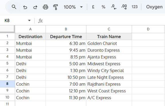
Consider a sample train schedule with destination, departure time, and train name or number. We will extract the earliest train to each location and the latest train to each location.
Sample Data
1. Retrieve the Earliest Entry Per Category in Google Sheets
Assume the above train schedule is in A1:C.
- The category is the destination in column A.
- To extract the earliest train for each destination, use the following formula:
=SORTN(SORT(A2:C, 1, TRUE, 2, TRUE), 9^9, 2, 1, TRUE)Earliest Train to Each Destination:
| Destination | Departure Time | Train Name |
| Cochin | 7:00 am | Rajdhani Express |
| Delhi | 5:00 am | Midwest Express |
| Mumbai | 6:30 am | Golden Chariot |
Formula Explanation
This formula combines SORT and SORTN:
SORT:
SORT(A2:C, 1, TRUE, 2, TRUE)- Sorts the train schedule first by destination (column 1, ascending) and then by departure time (column 2, ascending).
- This arranges the table so that the earliest train appears first for each destination.
SORTN:
=SORTN(..., 9^9, 2, 1, TRUE)- Extracts the first occurrence of each category (destination) from the sorted list.
- Ensures that only the earliest train per category is selected.
Tip: Modify the column numbers in the formula (highlighted) to match your dataset if your category or time column is in a different position.
2. Retrieve the Latest Entry Per Category in Google Sheets
To extract the latest train for each destination, we only need to change one thing:
Modify the SORT function to sort the time column in descending order (replace TRUE with FALSE for the second sorting criteria).
Updated Formula:
=SORTN(SORT(A2:C, 1, TRUE, 2, FALSE), 9^9, 2, 1, TRUE)Latest Train to Each Destination:
| Destination | Departure Time | Train Name |
| Cochin | 11:30 pm | A/C Express |
| Delhi | 10:50 pm | Late Night Express |
| Mumbai | 8:15 pm | Ajanta Express |
Does This Formula Work with Timestamps or Dates?
Yes! This method works for extracting the earliest or latest entry per category based on time, date, or datetime values.
If you need:
- To find the last row in each group without sorting by date, check this post.
- To extract the last entry by date, check this post.
Conclusion
We have seen one of the simplest formulas to extract the earliest or latest record per category in Google Sheets.
Key Takeaways:
- We used the SORTN function’s duplicate removal feature to achieve this.
- The SORT function is optional if you manually sort your data (Data > Sort range), but using SORT ensures your source data remains unaltered.
- This method works for time, date, and datetime columns in Google Sheets.
Now you can apply this to your own datasets and automate earliest/latest data retrieval in Google Sheets!


It is super helpful!
How can I retain the first entry within a month but also show the unique data?
Hi, Marlon Rafael Orpilla,
It’s not clear whether you have data spread across several months.
If you want me to look into this problem, please make a sample sheet with enough sample data and share that link/URL via ‘reply’ below.
I won’t publish that link.
This is super helpful! How can I do that, remove the duplicates from one column, leaving only the most recent date, but also show the data sorted by 2 sort ranges?
Hi, Jessica Gonzalez,
Use SORTN as explained. Then wrap the output with SORT to sort by two sort ranges.
If you want more clarification, please do leave your sample sheet URL in the reply.
This is very helpful. Thank you. How can we find the second-highest value based on the timestamp? Is it possible with the Sortn function?
A single value or values from each group?
Values from each group. Just like you got in the above example. Instead of values based on the last timestamp, I am looking for the second last timestamp values. I have values entered from a counter every hour. I am trying to find the difference between the last and the second last to get whatever was incremented in the last hour.
Hi, Usman Obaid,
I’ve published a new tutorial that may fulfill your requirement.
How to Find Second Highest Value from Every Group in Google Sheets.