If you’re working with running totals—like daily sales, expenses, or donations—you might want to find the exact row where your target is first reached. That’s where this little trick using SCAN and XMATCH comes in handy.
You can use it to return the target sum reached row in Google Sheets, either as the actual row number or just the relative position within your range.
Why Find the Target Sum Reached Row?
Let’s say you’re tracking sales day by day and want to know when you hit your monthly target. Once the running total reaches or exceeds your goal, you might want to:
- Pull related data from that row (like the date)
- Highlight it in a chart
- Or trigger other calculations
To do that, you first need to find the row where the target sum is reached.
Sample Setup
You have:
- Dates in column A →
A2:A - Sales volumes in column B →
B2:B - A target amount (say 200) in cell
D2
Now let’s find the row where the running total reaches or passes that target.
Formula to Find Target Sum Reached Row in Google Sheets
Here’s the formula:
=XMATCH(D2, SCAN(0, B2:B, LAMBDA(acc, val, acc + val)), 1) + ROW(B2) - 1How This Formula Works
Let’s break it down step by step:
SCAN(0, B2:B, LAMBDA(acc, val, acc + val))
This part creates a running total of the values in column B. It accumulates each value on top of the previous total, row by row.XMATCH(D2, ..., 1)XMATCHsearches the running total for the first value that’s greater than or equal to the target in cellD2. The1at the end tells it to find the smallest value that is greater than or equal to the target.+ROW(B2) - 1
SinceXMATCHreturns the position within the range (starting from 1), we addROW(B2) - 1to convert it into the actual row number on the sheet.
If you only need the position within the range and not the actual sheet row number, you can remove the last part:
=XMATCH(D2, SCAN(0, B2:B, LAMBDA(acc, val, acc+val)), 1)Example
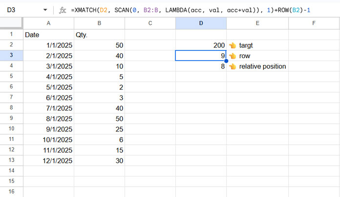
If you enter 200 in cell D2, the formula will return row 9, which is where the running total first hits or passes the target.
If you remove +ROW(B2)-1, you’ll get 8, which is the position in the range B2:B.
What If the Target Isn’t Reached?
If the values in B2:B never add up to the target in D2, the formula will return #N/A.
Bonus: Lookup a Value When the Target Is Reached
Finding the row is often just the first step. You might also want to return a value from another column, like the date or a label, once the target is hit.
Instead of using the row number with INDEX, you can use XLOOKUP directly with the running total.
Get the Date When the Target Is Reached
=XLOOKUP(D2, SCAN(0, B2:B, LAMBDA(acc, val, acc + val)), A2:A, "Target is not reached!", 1)This pulls the corresponding date from column A.
Get the Reached Total Itself
You can also return the cumulative total when the target is hit:
=XLOOKUP(D2, SCAN(0, B2:B, LAMBDA(acc, val, acc + val)), SCAN(0, B2:B, LAMBDA(acc, val, acc + val)), "Target is not reached!", 1)To make it cleaner and avoid repeating the SCAN function, wrap it in LET:
=LET(rs, SCAN(0, B2:B, LAMBDA(acc, val, acc + val)), XLOOKUP(D2, rs, rs, "Target is not reached!", 1))This is more efficient and easier to maintain.


Thanks, Prashanth, that works. The last problem is when the target sum isn’t reached.
Is there a way to pick a value to return in this case?
It currently attempts to output an array: “Array result was not expanded because it would overwrite data in XX.”
Hi, Brad Garcia,
I couldn’t replicate that issue on my end. Can you please share a sample?
Hi Prashanth,
Here’s a small example: * removed by admin *
Hi, Brad Garcia,
If there is no match (doesn’t reach the target sum), the formula returns #N/A. To remove that, you have placed the IFNA around XMATCH. INDEX reads it as
=index(A2:A,,1).So place IFNA() outside the INDEX.
Thanks Prashanth! That works!
Thanks Prashanth. This article is almost exactly what I need.
I have one more contstraint. I have an additional comment that is either blank, or has an “x”. I would like to limit the rows being added together to be the ones where that entry has an “x” in this additional column.
I tried changing SUMIF to SUMIFS (as well as moving the 3rd argument to be the 1st argument), but that resulted in the error message “Array arguments to SUMIFS are of different size.” Is it possible to add this additional constraint?
HI, Brad Garcia,
Thanks for your feedback. The SUMIFS won’t work that way. We can use a LAMBDA formula to replace the running total SUMIF.
Also, we require replacing MATCH with XMATCH.
My sample data is as follows.
A2:A – Dates
B2:B – Amount
C2:C – Contains “x” or blank.
F2 – Lookup amount (target sum).
Formula:
=index(A2:A,xmatch(F2,
if(C2:C="x",scan(0,if(C2:C="x",B2:B,0),lambda(a,v,a+v))),
1))
Resources:
1. Conditional Running Total.
2. XMATCH.