You can use three primary formulas to find the cell address of a lookup value in Google Sheets: VLOOKUP, XLOOKUP, and a combination of INDEX and MATCH. While VLOOKUP can be useful, XLOOKUP is generally more versatile.
These formulas don’t directly return the cell address but can be used with the CELL function to determine the cell location. There is an info type called “address” in the CELL function, which helps us return the cell address of a specified cell.
Syntax: CELL(info_type, reference)
Example:
=CELL("address", B9)The above formula would return $B$9 (cell address).
The CELL function supports an expression (a formula) as a reference instead of a direct reference to a cell.
This opens the possibility of using the CELL function to return the cell address of a lookup value.
How?
We will use a lookup formula as the reference within CELL. I will elaborate on that in the sections below.
Finding the Cell Address of a Lookup Value in Google Sheets
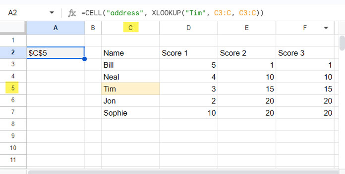
We have sample data in the range C2:F, where C2:C contains the names of players. I want to look up the name of a player, “Tim,” and return the cell address of that name.
Solution 1: XLOOKUP
=CELL("address",
   XLOOKUP("Tim", C3:C, C3:C)
)
The XLOOKUP function searches for the name “Tim” in the lookup range C3:C and returns the result from the result range, which is also C3:C. The CELL function then returns the “address” of this value.
You might wonder why not use VLOOKUP. The reason is that it won’t work in this case. If the lookup value and the result value are from the same column, the CELL function will return the error #N/A (“argument must be a range”).
Solution 2: INDEX-MATCH
=CELL("address",
   INDEX(C3:C, MATCH("Tim", C3:C, FALSE))
)
In this formula, the MATCH function returns the relative position of the lookup value “Tim” in C3:C. The INDEX function uses that position to return the value from the range C3:C. Wrapping it with the CELL function will return the cell address of the lookup value.
Finding the Cell Address of a Lookup Result Value in Google Sheets
With a slight modification to the formulas above, you can find the cell address of the lookup result value.
Example:
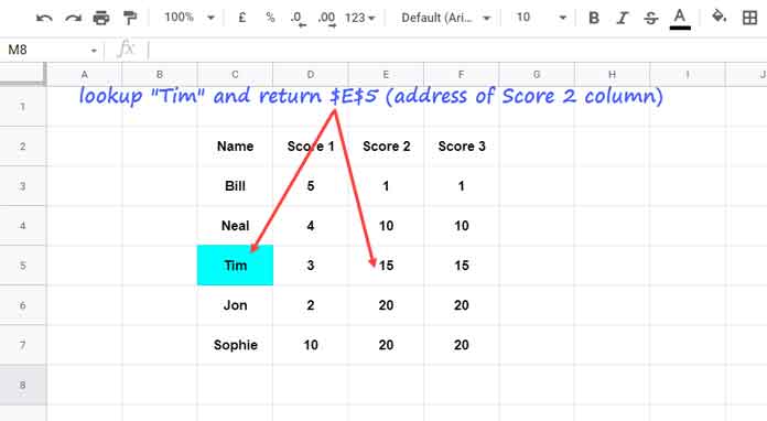
If you want to search for the name “Tim” in C3:C and get his score from E3:E, and then find the cell address of that result:
For XLOOKUP, replace the result range in the earlier formula (C3:C) with E3:E:
=CELL("address",
   XLOOKUP("Tim", C3:C, E3:E)
)
For INDEX-MATCH, replace the offset range C3:C with E3:E:
=CELL("address",
   INDEX(E3:E, MATCH("Tim", C3:C, FALSE))
)
VLOOKUP will also work:
=CELL("address",
   VLOOKUP("Tim", C3:F, 3, FALSE)
)
In this formula, VLOOKUP searches for “Tim” in the first column of the range C3:F and returns the result from the 3rd column. The CELL function then returns the cell address.
Cell Address of the Lookup Intersection Value in Google Sheets
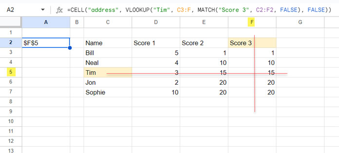
Sometimes you may want to find the cell address of the intersection value between two lookups. For example, you might want to search for the name “Tim” in A3:A and “Score 3” in C2:F2 and return the intersection value.
In that case, you can use either VLOOKUP or INDEX-MATCH with CELL.
VLOOKUP:
=CELL("address",
   VLOOKUP("Tim", C3:F, MATCH("Score 3", C2:F2, FALSE), FALSE)
)
This formula searches for “Tim” in column A (A3:A) and “Score 3” in row 2 (C2:F2), then returns the cell address of the intersecting value in the range C3:F.
INDEX-MATCH:
=CELL("address",
   INDEX(C3:F, MATCH("Tim", C3:C, FALSE), MATCH("Score 3", C2:F2, FALSE))
)
In this formula, the INDEX function returns the value at the intersection defined by the row and column numbers provided by the two MATCH functions. The CELL function then returns the address of that value.
Error Handling
#N/A is the most common error you may encounter when using the above formulas. It usually occurs when the search key (lookup value) is not present in the lookup range.
This might be due to a typo in specifying the search key in the formulas, so check for that first. To handle this error, you can wrap the formula with the IFNA function.


