The Lookup function can’t return a multiple column output. In this post last row lookup and array result in Google Sheets, I am going to give you some alternative formulas for the same.
I have 4 different formula options to replace Lookup to return an array result in Google Sheets. Before coming to that let me clear your doubts first.
Actually we can rewrite the topic to ‘Lookup Array Result in Google Sheets’. But I have decided to include the term ‘Last Row’ with the title purposefully.
The following example is meant for clearing up your doubts related to the last row lookup. Before that here is the Lookup function syntax for your quick reference.
Syntax 1:
LOOKUP(search_key, search_range, result_range)
Syntax 2:
LOOKUP(search_key, search_result_array)
I am following Syntax 1 in my example but applicable to Syntax 2 also (yes! we can use the Lookup function in two different ways).
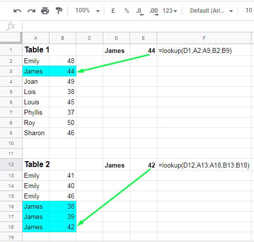
In my example, there are two tables and two Lookup formulas. In both the formulas, the search key to lookup is “James”.

search_key = D1 (formula 1) | D12 (formula 2)
search_range = A2:A9 (formula 1) | A13:A18 (formula 2)
result_range = B2:B9 (formula 1) | B13:B18 (formula 2)
The Lookup formulas look through column A (search_range) for the key “James” and return the value from the result_range (column B). Please note, the data must be sorted.
Since there are duplicates in the second table, the Lookup in the cell E12 returns a value from the last row from result_range. I hope now it may clear to you why I have used the term ‘last row lookup’.
Last Row Lookup and Array Result in Google Sheets – Formula Options
In result_range in Lookup, we can only use a single column (or single row). That means we can’t get an array result from a single Lookup formula in Google Sheets.
Here comes the topic Last Row Lookup and Array Result in Google Sheets relevant.
Brushup your last row lookup skill in Google Sheets. Below you can find 4 formulas to lookup the last row and return array results (multiple column results) in Google Sheets.
I have 4 different types of formulas for last row lookup and to return an array result. In that, one formula is based on QUERY and in all the other three formulas the FILTER function is the key.
It’s like Filter + Index (formula 1), Filter + Vlookup (formula 2), Filter + Sortn (formula 3) and finally the Query (formula 4).
Please find the formulas and the usage notes (formula explanations) below.
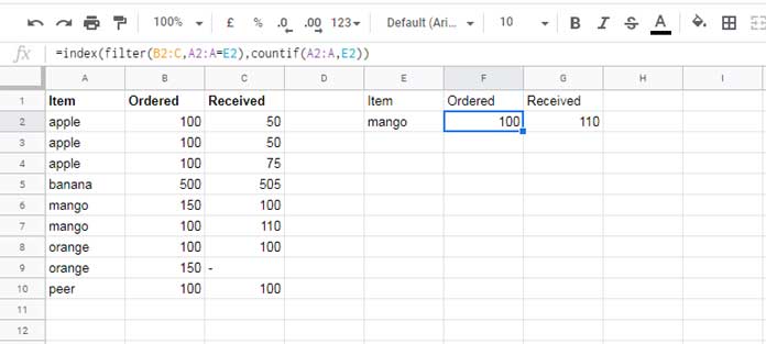
My sample data contains fruit names and their “Ordered” and “Received” quantities. A fruit may have multiple orders. What I want is to find the last ordered and received quantities of any particular fruits.
This we can achieve by lookup the fruit name in the last row (contains the last order). Let me start with the Filter Index combo.
Please do note that, unlike in Lookup function, in the combos, you can use sorted or an unsorted list. The formulas itself will take care of the data order. Anyway, I am using a sorted range in my examples.
Index and Filter (Formula 1)
In all the 4 formula examples to last row lookup and array result in Google Sheets, I’ll use the below same sample data and criterion. The only changes will be in the formula in cell F2.

The search key is the fruit name “mango”. I want to find the last ordered and received quantities of this item which are in row # 7.
Formula:
=index(filter(B2:C,A2:A=E2),countif(A2:A,E2))Explanation:
The Filter formula filters the rows containing the fruit name “mango”.
=filter(B2:C,A2:A=E2)Only the columns B and C (B2:C) included in the filter range. So all the ordered and received quantities of the fruit “mango” will be filtered as below.
| 150 | 100 |
| 100 | 110 |
These quantities are from rows 6 and 7. Now we just need to extract the last row. For that, I have used the Index function.
Syntax: INDEX(reference, [row], [column])reference – In the Index, I have used the above filter formula as the ‘reference’.
row – Since there are two rows in the filter result we must specify 2 (last row) as the ‘row’ to return. The Countif does that part.
column – Since we need all the columns, I have omitted the ‘column’ argument.
We can use the above formula option # 1 for last row lookup and array result in Google Sheets.
In the next two formulas, I am using the ‘same’ above Filter formula. I am going to only replace Index with Sortn and Vlookup respectively.
Vlookup and Filter (Formula 2) – Recommended
Even though the Index and Filter combo is easy to follow, some of you may not want to use the above formula (some users don’t want to use Index). Then the better one is Vlookup and Filter.
Syntax: VLOOKUP(search_key, range, index, [is_sorted])How to write the formula?
search_key – E2
range – filter formula above. Here there is a minor change in the filter formula and subsequently in its output.
The filter range is A2:C, not B2:C as earlier.
=filter(A2:C,A2:A=E2)So the result will be as follows.
| mango | 150 | 100 |
| mango | 100 | 110 |
index – {2,3}. We want columns 2 (Ordered) and 3 (Received) in the output.
Here is my recommended Vlookup formula for last row lookup and array result in Google Sheets. The ArrayFormula is included since the result that we want is an array.
=ArrayFormula(vlookup(E2,filter(A2:C,A2:A=E2),{2,3},1))Sortn and Filter (Formula 3)
This is the third combo to lookup the last row and to return an array result in Google Sheets.
I am not recommending this combo but included as part of my effort to give you all possible options. Also, I hope, this will help you understand how useful is Sortn.
Here let us use the Filter formula used in Formula 1, not in Formula 2. First, see the formula (Sortn + Filter). Then I’ll explain it.
=sortn(filter(B2:C,A2:A=E2),1,0,sequence(countif(A2:A,E2),1),0)I may require to use the syntax of Sortn to explain the formula. Before that, let me explain the logic behind the Sortn and Filter combo to lookup the last row and return an array in Google Sheets. It’s like this.
The filter formula filters the rows containing “mango” which is the search key. The Sortn sorts this data in descending order and returns 1 row (first row).
Here there is one issue. There is no meaning of sorting a filtered output by fruit names as it will only contain one fruit name.
Then how to sort the filtered fruits in descending order to get the last row as the first row?
To sort the data in descending order I have used sequential numbers generated by a Sequence function based formula.
Go through the syntax and arguments explanation below to understand the Sortn + Filter combination.
Syntax: SORTN(range, [n], [display_ties_mode], [sort_column], [is_ascending], [sort_column2, …], [is_ascending2, …])range – filter formula.
n – 1 (sorted ‘n’ rows). We just want the first row after sorting the data in descending order.
display_ties_mode – 0 (learn display ties mode)
sort_column – sequence(countif(A2:A,E2),1). This formula returns 2 rows (Countif formula) and 1 column which is the sort order.
| 1 |
| 2 |
is_ascending – 0 (sort the sort_column in descending order)
Query Formula to Lookup Last Row and Return Array Result in Google Sheets (Formula 4)
Here is the 4th formula for the last row Lookup and array result (multiple column result) in Google Sheets.
=query(A2:C,"Select B,C where A='"&E2&"' offset "&countif(A2:A,E2)-1)This formula filters the row containing the criterion “mango” and then offset 2-1 (Countif – 1) rows.


