The XLOOKUP function in Google Sheets is not inherently designed as a multiple-criteria function. However, we can adapt it to handle multiple criteria using IF and Boolean logic.
While the regular XLOOKUP can take one or more search keys, searching them in a column of a range and returning corresponding value(s) from another column, it may not directly support searching for one key in one column and another key in a different column, with both needing to match in the same row.
This scenario, known as XLOOKUP with multiple criteria, can be addressed by implementing IF and Boolean logic in Google Sheets. Let’s explore a few examples.
XLOOKUP with Multiple Criteria: Exact Match
In columns A to D, where A1:D1 contains field labels, we have item names, purchase dates, purchase months, and prices. Refer to the sample data in the screenshot below or click on the link below the image to copy the sample sheet.
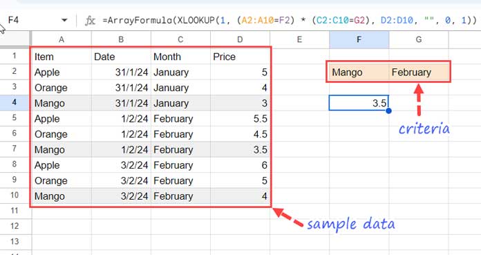
The items, such as “Apple,” “Orange,” and “Mango,” appear multiple times in the table.
Now, suppose we want to find the price of Mango in February by searching from top to bottom in the table. Our criteria are stored in F2 and G2, where F2 contains “Apple,” and G2 contains “February.”
Here is the formula to use (visible in the formula bar in the screenshot above).
Formula:
=ArrayFormula(XLOOKUP(1, (A2:A10=F2) * (C2:C10=G2), D2:D10, "", 0, 1))Formula Breakdown:
This follows the XLOOKUP syntax: XLOOKUP(search_key, lookup_range, result_range, [missing_value], [match_mode], [search_mode])
Where:
search_key: 1lookup_range: (A2:A10=F2) * (C2:C10=G2)result_range: D2:D10missing_value: “”match_mode: 0 (exact match)search_mode: 1 (Search from the first value to the last value; use -1 to search from the last value to the first.)
The logic in this multiple criteria XLOOKUP is straightforward.
The lookup_range in XLOOKUP must be a single column or row, but in our case, we need to look up in two columns: column A contains items, and column C contains months.
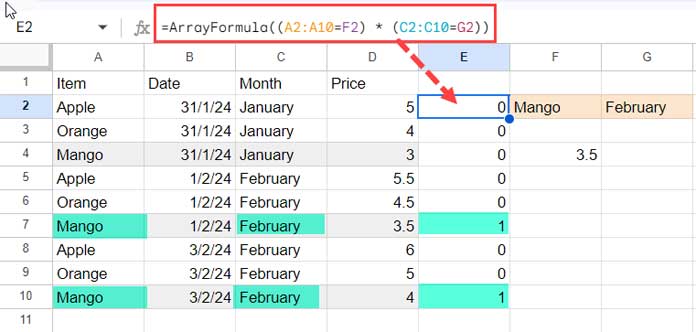
To resolve this, we merge both criteria columns into a single column using (A2:A10=F2) * (C2:C10=G2) in the lookup_range. The use of the ARRAYFORMULA function with XLOOKUP is necessary because this Boolean logic requires array formula support.
(A2:A10=F2): Returns TRUE wherever the first criterion (“Mango”) matches; otherwise, returns FALSE.(C2:C10=G2): Returns TRUE wherever the second criterion (“February”) matches; otherwise, returns FALSE.
The multiplication of TRUE x TRUE is 1. Essentially, the lookup_range returns a column with 1 or 0, and that’s why we use 1 as the criterion.
XLOOKUP with Multiple Criteria: Approximate Match
In the previous example, we explored the usage of XLOOKUP with multiple criteria for exact matches.
The formula can be applied to search either from the first value to the last value or vice versa in the table. By replacing the search mode with -1 in the formula, you can change the direction of the search.
Now, let’s delve into an example involving an approximate match, utilizing match mode 1 or -1 (instead of 0 in our previous example).
Suppose we want to find the price of Mango (F2) received on 02/02/2024 (G2) or, if there is no receipt, on the next available latest date. How can we achieve this?
Formula:
=ArrayFormula(XLOOKUP(G2, IF(A2:A10="Mango", B2:B10), D2:D10, "", 1, 1))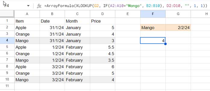
This represents an instance of XLOOKUP with multiple criteria and an approximate match in Google Sheets.
In this scenario, the search_key is the date criterion in cell G2, and the result_range is D2:D10.
The lookup_range is provided by IF(A2:A10="Mango", B2:B10), yielding a column with the corresponding date against the item Mango and FALSE in all other rows.
In this column (the values returned by the IF logical test), XLOOKUP can execute an approximate match of the search key, which is the date in G2.
Now, to find the price of the Mango (F2) received on 02/02/2024 (G2) or, if there is no receipt, on the next available earliest date, replace match mode 1 with -1 in the formula:
=ArrayFormula(XLOOKUP(G2, IF(A2:A10="Mango", B2:B10), D2:D10, "", -1, 1))Here, you can also direct the formula to search from the bottom to the top by replacing the last argument in the formula with -1.
XLOOKUP with Multiple Criteria: Partial Match
For a partial match, we need to use match mode 2 in XLOOKUP. However, in an XLOOKUP with multiple criteria, using match mode 2 directly is not feasible.
Instead, we can utilize REGEXMATCH or SEARCH when merging multiple lookup columns into a single one. I prefer using SEARCH as it appears to be relatively simpler.
Let’s consider a scenario where we have various grade labels for fruits in column A. Instead of the item “Mango,” we have variations like “Mango MG-A,” “Mango MG-EQ,” “Mango OG-M,” etc.
Now, if we want to look up the price of Mango received in January, the formula would be:
Formula:
=ArrayFormula(XLOOKUP(1, SEARCH(F2, A2:A10) * (C2:C10=G2), D2:D10, "", 0, 1))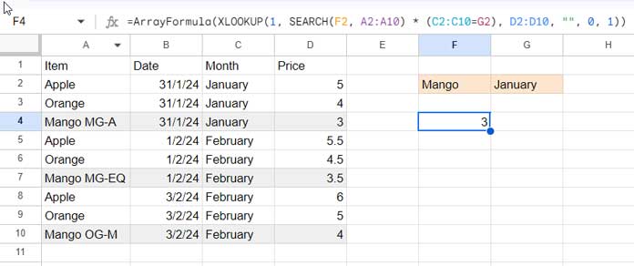
This multiple criteria XLOOKUP operates as follows:
- The search key is 1, indicating the adoption of Boolean logic in the lookup range.
- The lookup_range is
SEARCH(F2, A2:A10) * (C2:C10=G2). Here, SEARCH returns 1 wherever it partially matches the first criterion in the item column. The second part,(C2:C10=G2), matches the month in the month column and returns TRUE or FALSE. - When multiplying, the formula returns 1 or 0, and we are looking up 1.
In the context of this table, if you wish to find the price of Mango received on 02/02/2024 or the next latest available date, you can use the following formula:
=ArrayFormula(XLOOKUP(G2, IF(SEARCH(F2, A2:A10)=1, B2:B10), D2:D10, "", 1, 1))This follows the IF logic, which we used in the approximate match. In that case, we used IF(A2:A10="Mango", B2:B10) as the lookup range. Here, we incorporate the SEARCH function and use IF(SEARCH(F2, A2:A10)=1, B2:B10) as the lookup range.
Conclusion
This tutorial covered how to use XLOOKUP with Multiple Criteria in Google Sheets.
If you want to explore more XLOOKUP examples in Google Sheets, including beginner tutorials, advanced lookup techniques, and real-world use cases, check out the Complete Guide to XLOOKUP in Google Sheets.


