This tutorial guides you through harnessing the capabilities of XLOOKUP to fetch results spanning multiple columns and rows in Google Sheets. We’ll make XLOOKUP even more versatile by addressing one of its limitations.
A drawback of XLOOKUP compared to VLOOKUP lies in its array formula capability—it can return multiple column results, but only for a single search key.
When your search keys are organized in a column, attempting to conduct a lookup and retrieve multiple column results for all keys poses a challenge, and even the use of ARRAYFORMULA won’t make a difference. In such scenarios, VLOOKUP performs admirably.
Despite the lookup capabilities, we can’t entirely replace XLOOKUP with VLOOKUP. Instead, we need to find a solution to make XLOOKUP work seamlessly for multiple columns and rows in Google Sheets.
Discover two effective approaches in this tutorial: utilizing the MAP lambda function to iterate over search keys or BYCOL to iterate over the columns in the result range.
Let’s dive into the first solution—XLOOKUP for multiple-column results using MAP in Google Sheets.
XLOOKUP: Multiple Column Results with MAP in Google Sheets
We have a three-column table in Google Sheets containing the employee’s name, salary, and department. The range is B2:D7, where B2:D2 contains the labels “Employee,” “Salary,” and “Department.”
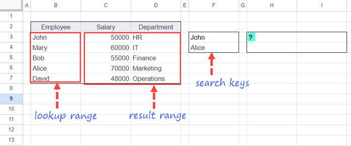
To look up an employee’s name in cell F3 and return both their salary and department, you can use the following XLOOKUP formula in cell H3:
=XLOOKUP(F3, B3:B7, C3:D7)Where:
search_key: F3lookup_range: B3:B7result_range: C3:D7
But what if you have employee names in both F3 and F4?
You might think that replacing F3 with F3:F4 and entering the formula as an array formula would yield the desired result. However, this is not the case.
The following XLOOKUP array formula will return only the salary column, even if the lookup range contains both salary and department.
=ArrayFormula(XLOOKUP(F3:F4, B3:B7, C3:D7))To handle this scenario, you can use the MAP function with XLOOKUP to return multiple-column results in Google Sheets:
=MAP(F3:F4, LAMBDA(val, XLOOKUP(val, B3:B7, C3:D7)))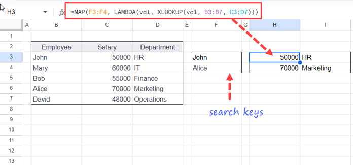
Within MAP, we’ve specified the search key range to iterate over each value in it. Each value is represented by val. In the XLOOKUP function, instead of F3:F4, we’ve specified val to dynamically reference the varying search key range.
XLOOKUP: Multiple Column Results with BYCOL in Google Sheets
In the example above, we utilized the MAP lambda function with XLOOKUP for obtaining multiple-column results. Now, let’s explore the BYCOL alternative.
=ArrayFormula(BYCOL(C3:D7, LAMBDA(col, XLOOKUP(F3:F4, B3:B7, col))))The BYCOL function employs the result range C3:D7 and iterates over each column in this 2D array. Each column is represented by col. Therefore, in the XLOOKUP function, we use col instead of the result range C3:D7.
Note that ARRAYFORMULA support is required, as XLOOKUP necessitates it when handling multiple search keys in a single-column result range.
BYCOL vs. MAP for XLOOKUP Array Result: Making the Right Choice
Both BYCOL and MAP are Lambda helper functions (LHF), and both can impact spreadsheet performance, especially with large datasets.
Determining the most efficient function ultimately depends on your specific data and function. However, there are considerations based on the nature of your data.
Here’s a guideline for choosing the right lambda function to use with XLOOKUP for multiple-column results:
- If you have a smaller number of search keys compared to the number of rows in the lookup range, opt for MAP.
- For a larger number of search keys, consider using BYCOL.
Why Shouldn’t We Consider Alternatives to XLOOKUP for Multiple Column Results?
Some of you may wonder why we don’t opt for FILTER or QUERY as alternatives to look up multiple search keys and return multiple-column results.
The main reason is the XLOOKUP capability to search from the first value to the last value and vice versa.
Additionally, XLOOKUP can perform exact matches and approximate matches. It can also be customized, such as using less than or equal to the search key or greater than or equal to the search key.
Moreover, if we have three search keys and the second search key has no matching value, we can identify this because XLOOKUP will leave #N/A or a placeholder with the value we specified in the formula. However, when employing FILTER or QUERY, this won’t be possible.
One alternative I can suggest is a formula that uses XMATCH. It has one drawback, namely the missing value mentioned above. You can read more about it in my CHOOSEROWS function guide.
In the above example, we can use the following formula as an alternative to XLOOKUP for multiple-column results:
=ArrayFormula(CHOOSEROWS(B3:D7, TOCOL(XMATCH(F3:F4, B3:B7), 3)))In this formula, XMATCH returns the relative position of the search keys in the lookup range, and CHOOSEROWS selects those rows. The formula is set to return all three columns.
Conclusion
This tutorial covered how to use XLOOKUP for Multiple Column Results in Google Sheets.
If you want to explore more techniques like this, visit our Complete Guide to XLOOKUP in Google Sheets, where we compile practical XLOOKUP examples in Google Sheets ranging from beginner formulas to advanced lookup strategies.


Brilliant article!