Removing milliseconds from timestamps is an important technique to be aware of in Google Sheets, as it can help troubleshoot formula errors.

For instance, if you used keyboard shortcuts to insert static timestamps in Google Sheets, they might appear like timestamps without milliseconds.

However, if you select those cells and apply DD/MM/YYYY HH:mm:ss.000 in Format > Number > Custom number format, you will reveal the actual underlying values.

As a result, issues may arise when performing lookups or using other criteria that involve matching in the timestamp column.

Your criterion or search key may be a timestamp in the formula, such as DD/MM/YYYY HH:mm:ss, without milliseconds, to find an exact match. However, the search column will contain timestamps with milliseconds.

In this walkthrough, you can learn how to remove milliseconds from timestamps in a column in Google Sheets. For that, we will use both array and non-array formulas.

We will use two types of formulas.

The first formula will simply truncate the milliseconds and return the timestamp without milliseconds. For example, if the timestamp is 13/08/2023 08:47:08.704, the formula will return 13/08/2023 08:47:08.

The second one will round up the seconds. For example, if the timestamp is 13/08/2023 08:47:08.704, the formula will return 13/08/2023 08:47:09. If the milliseconds are less than 500, the formula doesn’t change the seconds’ value; otherwise, it adds 1 to the seconds’ value.

You can choose the formula you prefer.

Removing Milliseconds from Timestamps in Google Sheets

If you want to truncate the milliseconds from timestamps, follow this approach.

Assume you have the timestamp in cell A2. You can use the following formula in any other cell to remove the milliseconds without making any other changes to the timestamp.

=A2-QUERY(A2, "Select millisecond(A) label millisecond(A)''", 0)/86400000

Note: You may need to format the result of this formula and the formulas below to the timestamp format using Format > Number > Date time.

The QUERY function is used to extract the milliseconds part of the timestamp in cell A2.

For instance, if the value is 13/08/2023 08:47:08.704, the formula will return 704. To remove the milliseconds from the timestamp in cell A2, it’s necessary to convert this value into the equivalent fraction of a day.

Therefore, the extracted milliseconds value is divided by 86400000, which represents the number of milliseconds in a day. Subtracting this calculated fraction from the original timestamp results in a timestamp without milliseconds.

In summary, this formula effectively removes the milliseconds from the given timestamp in cell A2.

Can we use this in an array formula to remove milliseconds from a list in Google Sheets?

Absolutely! Here you go!

=ArrayFormula(
     IF(A2:A="", ,
     A2:A-QUERY(A2:A, "Select millisecond(A) label millisecond(A)''", 0)/86400000)
)

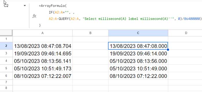
The ArrayFormula is used to apply the subtraction, division, and the IF logical test to the entire column.

The IF logical test ensures that the formula returns a blank in rows where there is no value in the list column (A).

Adjust Timestamps to the Nearest Second based on Milliseconds

Some of you may want to remove the milliseconds but round the seconds part. How do we adjust the timestamps to the nearest second based on milliseconds in Google Sheets?

For the timestamp in cell A2, you can use either of the formulas below:

=DATEVALUE(A2) + TIMEVALUE(TEXT(A2, "HH:mm:ss"))
=DATEVALUE(A2)+TIME(HOUR(A2), MINUTE(A2), SECOND(A2))

In both formulas, the DATEVALUE function returns the date value, while the TIME/TIMEVALUE functions return the time component.

In the first formula, the TEXT function is utilized to format the time as HH:mm:ss. The TIMEVALUE function then converts this time string into a time value. It’s important to note that removing milliseconds effectively rounds the seconds.

In the second formula, we use the HOUR, MINUTE, and SECONDS functions to retrieve the corresponding time components. The TIME function then converts those values into a time, and the SECONDS function is employed to round the seconds.

If the date in cell A2 is 05/10/2023 08:13:56.141, it will return 05/10/2023 08:13:56, truncating the milliseconds as they are below 500.

If the date in cell A2 is 19/09/2023 09:46:14.695, it will return 19/09/2023 09:46:15, rounding up the second.

You can use this in an array formula as well. Here is an example using the timestamps in A2:A:

=ArrayFormula(IFERROR(DATEVALUE(A2:A) + TIMEVALUE(TEXT(A2:A, "HH:mm:ss"))))
=ArrayFormula(IFERROR(DATEVALUE(A2:A)+TIME(HOUR(A2:A), MINUTE(A2:A), SECOND(A2:A))))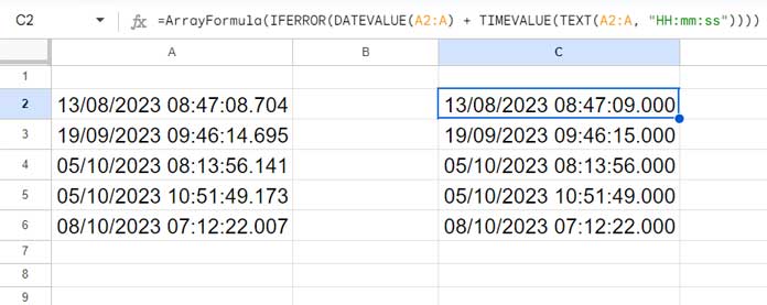

Here, ArrayFormula is used to support all the functions in use.

The IFERROR is employed to handle errors returned by DATEVALUE in blank cells. In blank cells, DATEVALUE returns an error, and we convert those errors to blanks using IFERROR. Therefore, the IF logic is not necessary.

Conclusion

We have explored two relatively simple solutions to remove milliseconds from timestamps in Google Sheets.

One truncates the timestamps, and the other removes the milliseconds but rounds the seconds based on the milliseconds.

Here are some resources about milliseconds in Google Sheets.

1. How to Extract Date From Timestamp in Google Sheets
2. How to Filter Timestamp in Query in Google Sheets
3. Extract the Earliest or Latest Record in Each Category Based on Timestamp in Google Sheets
4. How to Convert a Timestamp to Milliseconds in Google Sheets
5. Convert Unix Timestamp to Local DateTime and Vice Versa in Google Sheets
6. Vlookup Date in Timestamp Column in Google Sheets
7. How to Use Timestamp within IF Logical Function in Google Sheets
8. How to Insert a Static Timestamp in Google Sheets