This tutorial describes decoding or converting a Unix Timestamp to local DateTime in Google Sheets. For this purpose, Sheets offers a dedicated function called EPOCHTODATE.
In addition to the above how-to, I will explain how to convert a local DateTime to Unix Time, which is the reverse of the process described above.
I know many of you are familiar with or have heard of the terms Unix Time, Unix Timestamp, or Epoch Time. Essentially, all these refer to a 10-digit encoded UTC Date/DateTime.
Understanding Unix Time is crucial for writing a formula that converts Unix Timestamp to local DateTime or vice versa in Google Sheets.
Unix Time represents the seconds elapsed since 1st January 1970 (Epoch). As you may know, a standard day (in UTC) comprises 86,400 seconds (24 hours * 60 minutes * 60 seconds). These seconds play a vital role in the Unix Timestamp to local DateTime conversion formula in Google Sheets.
First, let’s outline the steps to convert a Local DateTime to Unix Time.
Converting Local DateTime to Unix Time in Google Sheets
To convert a local DateTime (Timestamp) in cell A2 to Unix Time, follow these steps in Google Sheets:
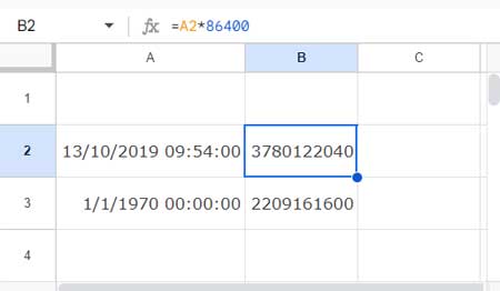
Example: A2 contains 13/10/2019 09:54:00
Step 1: Timestamps to Seconds
Convert the DateTime to the number of seconds by multiplying A2 by 86400, like this:
=A2*86400This formula in cell B2 will return 3780122040.
In cell A3, enter 1/1/1970 00:00:00 and convert this to seconds by multiplying A3 by 86400:
=A3*86400This formula in cell B3 will return 2209161600.
You might think that subtracting the seconds (B2-B3) will give you the Unix Epoch Time of the DateTime in A2, since Unix Time is the number of seconds since Epoch (1/1/1970 00:00:00). However, there’s an additional parameter to consider.
To accurately convert the local DateTime, consider the time zone. If the time in A2 is UTC, then using =B2-B3 will convert the Timestamp to Unix Time. If not, determine your local time zone offset.
Step 2: Unix Time Conversion from Local DateTime
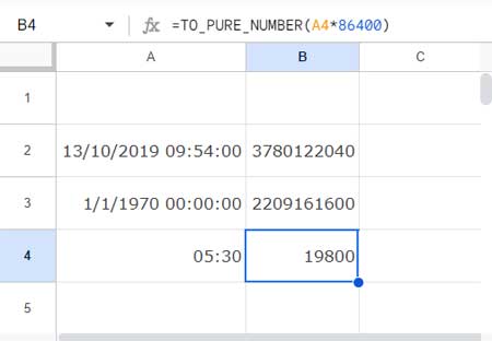
For instance, if the time in A2 is GMT+05:30 (India Standard Time), meaning five and a half hours ahead of UTC:
In cell A4, enter 5:30 (adjust this based on your local time zone).
In cell B4, use the following formula to convert the time zone offset to seconds:
=TO_PURE_NUMBER(A4*86400)This will convert 5:30 to 19800 seconds.
Step 3: Converting Local DateTime to Unix Time
Now, with the GMT Offset in seconds (cell B4), you can convert the local DateTime to Unix Time:
=B2-B3-B4So the Unix Time corresponds to the DateTime in cell A2, i.e., 13/10/2019 09:54:00, will be 1570940640.
Generic Formula:
In short, you can follow the below generic formula to convert a timestamp to Epoch Time in Google Sheets.
(DateTime-Epoch-GMT)*86400Note: If your timezone is GMT-, use the generic formula as:
(DateTime-Epoch+GMT)*86400In our example, you can use the formula as:
=(A2-A3-A4)*86400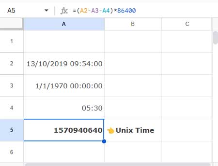
or
=(A2-DATE(1970, 1, 1)-TIME(5, 30, 0))*86400Converting Unix Timestamp to Local DateTime in Google Sheets
Once you’ve learned the conversion above, the reverse process—converting Unix Timestamp to local DateTime—is straightforward.
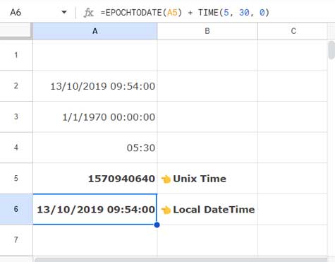
Here, the Unix Timestamp to convert to local DateTime is in cell A5, which is 1570940640.
First, convert the 10-digit Unix Time in seconds to DateTime by dividing Unix Time by 86400:
=A5/86400Then add Epoch Date Time and GMT to this DateTime:
=A5/86400 + DATE(1970, 1, 1) + TIME(5, 30, 0)Please note, if your timezone is GMT-, adjust the formula accordingly by subtracting the TIME(hr, min, sec).
With the new EPOCHTODATE function, you can replace the above formula with =EPOCHTODATE(A5) + TIME(5, 30, 0).
I hope this helps you understand how to convert Unix Timestamp to local DateTime and vice versa in Google Sheets.
Resources
- Extracting Date From Timestamp in Google Sheets: 5 Methods
- How to Extract Time from DateTime in Google Sheets: 3 Methods
- How to Compare Time Stamp with Normal Date in Google Sheets
- Converting Time Duration to Day, Hour, and Minute in Google Sheets
- How to Convert Military Time in Google Sheets
- Elapsed Days and Time Between Two Dates in Google Sheets
- Countdown Timers in Google Sheets (Easy Way!)
- How to Add Hours, Minutes, Seconds to Time in Google Sheets
- How to Format Time to Millisecond Format in Google Sheets
- How to Increment Time by Minutes or Hours in Google Sheets
- How to Convert a Timestamp to Milliseconds in Google Sheets
- How to Increment DateTime by One Hour in Google Sheets (Array Formula)
- How to Insert a Static Timestamp in Google Sheets
- How to Remove Milliseconds from Timestamps in Google Sheets


