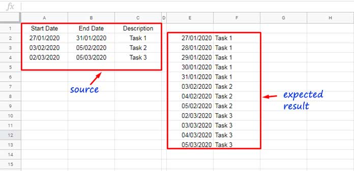
Expand Dates and Assign Values in Google Sheets (Array Formula)

How can we expand dates, like project start and end dates, and assign values, such as task names (for a project), in Google Sheets?

We can utilize SEQUENCE (for expanding dates) and VLOOKUP (for assigning values) in Google Sheets.

Alternatively, we can replace SEQUENCE with the ROW function. However, the SEQUENCE, being a relatively new function, is straightforward to use in this case.

Update:-

Expanding dates and assigning values becomes notably simpler with the introduction of the LAMBDA function in Google Sheets. I’ve included this solution at the end of the tutorial.

Expand Dates and Assign Values in Google Sheets – Old Method

Expand Dates and Assign Values in Google Sheets - Explained — image # 1

There are two drawbacks to expanding dates and assigning values using this old-school method (the method used before the launch of LAMBDA and associated helper functions) in Google Sheets. What are they?

The start date of “Task 2” must be greater than the end date of “Task 1,” and this condition applies to other tasks as well.
The “Description” column (Column C) must not be blank.

If you have two tasks that fall within the same period or overlap, the only option is to display the tasks as comma-separated.

Example:

Let’s say I have two tasks during the period from 02/03/2020 to 05/03/2020. I can represent them as follows:

Start Date	End Date	Description
02/03/2020	05/03/2020	Task 3, Task 4

If there are blank tasks, filter the data to a new range and use that data as the source:

=FILTER(A1:C, C1:C <> "")

If you find the above workarounds unsatisfactory, you can resort to helper tabs. Refer to the ‘Note’ tab in my sample Sheet at the end of this post for more information.

Steps

Here are step-by-step instructions for expanding dates and assigning values in Google Sheets.

You can find all the steps in my example Sheet, shared at the end of this post.

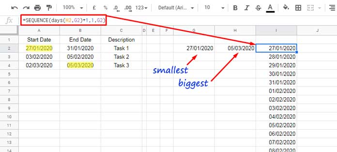
1. Find Min and Max Dates:

To obtain the smallest and largest dates in the range A1:B, start by entering the following formulas:

In cell G2: =MIN(A2:B)

In cell H2: =MAX(A2:B)

2. Expand the Min and Max Dates:

Generate a list of sequential dates (date values) between the minimum (G2) and maximum (H2) dates, inclusive:

In cell I2: =SEQUENCE(DAYS(H2, G2)+1, 1, G2)

Select the range I2:I and apply Format > Number > Date.

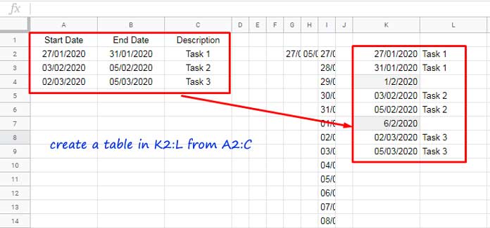
Expanding Dates Between Smallest and Largest Dates - Google Sheets — image # 2

3. Helper Table from Source Data:

Flatten the data in A2:B4 into columns K2:K, and copy-paste the corresponding tasks to L2:L.

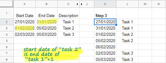
Insert one row after each task, and enter the dates that should be end_date_above + 1. Refer to the screenshot below for clarification.

Customized Start Dates and End Dates - Helper Table — image # 3

Notes:

If the start date of any task aligns with the end date of the previous task + 1, there is no need to insert a row.
Automation of this manual modification to the source data is achievable using a formula. Refer to cell K2 in the ‘Step 3 Also Auto’ tab for an example.

Important Point to Note When Expanding Dates and Assigning Values — image # 4

4. Vertical Lookup:

Insert the following VLOOKUP formula in cell J2.

=ArrayFormula(VLOOKUP(I2:I, K2:L, 2, 1))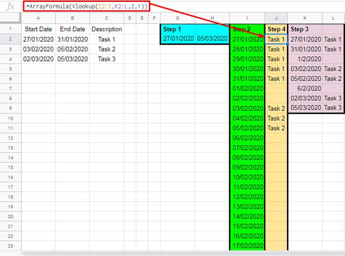

Raw Output of Exapnded Start/End Dates and Assigned Values (Tasks) in Google Sheets — image # 5

With this step, we have expanded dates and assigned values in Google Sheets.

Now, let’s combine the formulas and remove any unwanted rows from the result.

5. Combine Steps 1, 2, and 4 Formulas:

Here are the steps to combine formulas from Steps 1, 2, and 4.

First, combine Step 2 (I2) and Step 4 (J2) as follows in cell M2 (ignore any possible error):

={SEQUENCE(DAYS(H2, G2)+1, 1, G2), ArrayFormula(VLOOKUP(I2:I, K2:L, 2, 1))}

This is like {Step 2 Formula, Step 4 Formula}.

Then edit it and replace the cell references H2 and G2 with the formulas from the corresponding cells:

={SEQUENCE(DAYS(MAX(A2:B), MIN(A2:B))+1, 1, MIN(A2:B)), ArrayFormula(VLOOKUP(I2:I, K2:L, 2, 1))}

Make one more change to this formula. Replace I2:I with the I2 (Step 2) formula:

={SEQUENCE(DAYS(MAX(A2:B), MIN(A2:B))+1, 1, MIN(A2:B)), ArrayFormula(VLOOKUP(SEQUENCE(DAYS(H2, G2)+1, 1, G2), K2:L, 2, 1))}

Once again, edit it to replace the remaining cell references H2 and G2 with the corresponding formulas:

={SEQUENCE(DAYS(MAX(A2:B), MIN(A2:B))+1, 1, MIN(A2:B)), ArrayFormula(VLOOKUP(SEQUENCE(DAYS(MAX(A2:B), MIN(A2:B))+1, 1, MIN(A2:B)), K2:L, 2, 1))}

Finally, use QUERY to remove (filter out) unwanted rows (rows that do not contain tasks in the second column):

=QUERY({SEQUENCE(DAYS(MAX(A2:B), MIN(A2:B))+1, 1, MIN(A2:B)), ArrayFormula(VLOOKUP(SEQUENCE(DAYS(MAX(A2:B), MIN(A2:B))+1, 1, MIN(A2:B)), K2:L, 2, 1))},"SELECT * WHERE Col2 <>''")

Don’t forget to delete values in columns G to J. Keep the helper table (K2:L) as it is.

Expand Dates and Assign Values in Google Sheets – New LAMBDA Formula

Please scroll up and refer to image #1 for the sample data in cells A1:C1.

Below, you’ll find a new non-helper table method for expanding dates and assigning values in Google Sheets. I recommend using this solution over the previous method.

To implement this new approach, enter the following LAMBDA-based formula in cell E2 after clearing E2:F:

=ArrayFormula(SPLIT(TOCOL(MAP(A2:A, B2:B, C2:C, LAMBDA(a, b, c, IF(a*b, SEQUENCE(1, b-a+1, a)&"|"&c,))), 1), "|"))

Select E2:E and apply Format > Number > Date.

For an illustrative example, please refer to the ‘Lambda Eg 1’ tab in my sample Sheet.

Anatomy of the Formula and Logic

Retain only the sample data in cells A1:C in your Sheet. Let’s break down the formula step by step.

Initially, expanding two dates, for instance, A2 and B2, using the SEQUENCE function is straightforward. The challenge arises when replicating this operation in each row without manually dragging the formula down.

Place the following formula in cell D1 (it returns date values; disregard the formatting):

=IF(A2*B2, SEQUENCE(1, B2-A2+1, A2),)

To repeat this formula in each row within the range A2:C4, use the MAP Lambda Helper Function (LHF). In cell D1, enter:

=MAP(A2:A4, B2:B4, C2:C4, LAMBDA(a, b, c, IF(a*b, SEQUENCE(1, b-a+1, a),)))

Assign tasks to each date in the output by modifying it as follows:

=ArrayFormula(MAP(A2:A4, B2:B4, C2:C4, LAMBDA(a, b, c, IF(a*b, SEQUENCE(1, b-a+1, a)&"|"&c,))))

Ensure it is used as an array formula.

Flatten the output (multiple columns to one column) using the TOCOL function, which also filters out blank rows in one step:

=ArrayFormula(TOCOL(MAP(A2:A4, B2:B4, C2:C4, LAMBDA(a, b, c, IF(a*b, SEQUENCE(1, b-a+1, a)&"|"&c,))), 1))

Split the result into two columns at the “|” delimiter. Open the ranges A2:A4, B2:B4, and C2:C4 in the formula, respectively, to A2:A, B2:B, and C2:C.

Example Sheet

Hi again,

Actually, I managed to do the following to create the K & L columns in step 3:

Insert =COUNTA(A2:A) in Cell (G2) to calculate the Tasks’ row count.
Insert =$G$2*3 in Cell (G3) to calculate the final row count.

Tasks Row Count ==> 3 (G2)
Final Row Count ==> 9 (G3)

Then, inserted =ARRAY_CONSTRAIN(ARRAYFORMULA((B2:B4)+1),$G$2,1) in D2 to generate a populate the D columns with next date of the End Date. The result will be as follows:

Start Date (A) End Date (B) Description (C) Next Day (D)
27/01/2020 31/01/2020 Task 1 01/02/2020
03/02/2020 05/02/2020 Task 2 06/02/2020
02/03/2020 05/03/2020 Task 3 06/03/2020

Then, I inserted the following formulas in the cells shown below:

In Cell I2:
=ARRAY_CONSTRAIN(ARRAYFORMULA(IFERROR(VLOOKUP($K2:$K,{(A2:A),($C2:$C)},2,0))),$G$3,1)

In Cell J2:
=ARRAY_CONSTRAIN(ARRAYFORMULA(IFERROR(VLOOKUP($K2:$K,{(B2:B),($C2:$C)},2,0))),$G$3,1)

In Cell K2:
=ARRAY_CONSTRAIN(SORT(({ARRAYFORMULA(A2:A); ARRAYFORMULA(B2:B); ARRAYFORMULA(D2:D)})),$G$3-1,1)

In Cell L2:
=ARRAYFORMULA((I2:I10) & (J2:J10))

This produces the final result as shown in your example.

I hope this helps some readers!

Regards
Sabba

16 COMMENTS

Sabba June 17, 2020 At 5:12 pm

Hi Prashanth,

Thanks for your reply. Yes, your approach works. Thank you very much.

Kind regards

Sabba

- Prashanth October 26, 2022 At 2:55 pm
  
  Hi, Sabba,
  
  I’ve updated this post heavily. Please see the new LAMBDA solutions added by me that work without helper columns or tables.
  
Sabba June 11, 2020 At 9:38 pm

Hi Prashanth,

I am coming back to this tutorial. I do need to resolve the issue of duplicate dates. What I have now is the following problem, which I trust you can help.

A|B|C
Start Date|End Date|Timestamp
28/02/20|28/02/20|04/04/2020 17:12:26
06/03/20|06/03/20|06/03/2020 15:28:45
06/03/20|30/03/20|17/03/2020 13:55:36
13/03/20|13/03/20|05/03/2020 17:28:04
20/03/20|20/03/20|16/03/2020 12:55:05

I have used your below formula (maybe with some minor modifications):

=ArrayFormula(query({SEQUENCE(days(max(A2:B),min(A2:B))+1,1,min(A2:B)), ArrayFormula(Vlookup(SEQUENCE(days(max(A2:B),min(A2:B))+1,1,min(A2:B)), sort({Query({{A2:A,C2:C};{B2:B,C2:C}},"Select * "); iferror(if(indirect("B2:B"&match(1,B:B/B:B,1))+1= {iferror(indirect("A2:A"&match(1,B:B/B:B,1)),"");""}, {"",""},{iferror(indirect("B2:B"&match(1,B:B/B:B,1)),"")+1, iferror(indirect("B2:B"&match(1,B:B/B:B,1)),"")/0}),"")}, 1,1,2,1),2,1))},"Select * ",0))

This generates the following list:

E|F
Date|Timestamp
28/02/2020|04/04/2020 17:12:26
29/02/2020
01/03/2020
02/03/2020
03/03/2020
04/03/2020
05/03/2020
06/03/2020|17/03/2020 13:55:36
07/03/2020
08/03/2020
09/03/2020
10/03/2020
11/03/2020
12/03/2020
13/03/2020|05/03/2020 17:28:04
14/03/2020
15/03/2020
16/03/2020
17/03/2020
18/03/2020
19/03/2020
20/03/2020|16/03/2020 12:55:05
21/03/2020
22/03/2020
23/03/2020
24/03/2020
25/03/2020
26/03/2020
27/03/2020
28/03/2020
29/03/2020
30/03/2020|17/03/2020 13:55:36

As you will note the timestamp column is sparsely filled and mostly is left blank. What I really want is a list of dates with the oldest timestamp for duplicate dates and all dates have a timestamp associated with them. Timestamps are unique for each row.

Any thoughts? Your help is greatly appreciated.

Best regards.

Sabba

- Prashanth June 12, 2020 At 9:52 am
  
  Hi, Sabba,
  
  I guess you were trying to achieve the result with an array formula without helper columns.
  
  I’ve one example sheet at the end of this tutorial. In that, please open the tab named “Note” to read the notes. There, I’ve mentioned what to do when you have overlapping dates.
  
  I mean I may be able to solve this new puzzle with helper columns.
  
  Steps:
  
  Copy-paste your data (the date to expand with timestamp column instead of task column) in the range A1:C5 in the tab named as “1” (do not use the header row).
  
  Modify the formula in cell C1 in the tab named “2” as below.
  
  =sortn(sort(transpose({split(TEXTJOIN("|",true,'2'!A:A),"|"); split(TEXTJOIN("|",true,'2'!B:B),"|")}),1,1,2,1),9^9,2,1,1)
  
  See if that answers your problem.
  
  - Sabba June 12, 2020 At 5:10 pm
    
    Hi Prashanth,
    
    Many thanks for your prompt response.
    
    I tried your last formula, but it failed with this message:
    “In ARRAY_LITERAL, an Array Literal was missing values for one or more rows.
    
    Thanks again.
    Regard
    Sabbas
    
    - Prashanth June 13, 2020 At 9:04 am
      
      Hi, Sabba,
      
      I may require the file in EDIT mode, not VIEW. So please share your sheet again.
      
      Thanks.
      
      - Sabba June 13, 2020 At 4:13 pm
        
        Hi again,
        
        Shared it in edit mode;
        
        Best Regards
        Sabba
      - Prashanth June 14, 2020 At 10:11 am
        
        Hi, Sabba,
        
        It seems the given formula works. Please see your sheet for the new tabs 1 and 2.
        
        Best,
Sabba March 16, 2020 At 8:32 am

Hi Prashanth,

Your new formula works very well. I have used the following example:

Start date End date Description
10-03-2020 10-03-2020 Task 1
06-03-2020 10-03-2020
09-03-2020 12-03-2020 Task 1
15-03-2020 18-03-2020 Task 2
13-03-2020 14-03-2020 Task 3

Your formula produces the following result:

Date Description
06-03-2020 #N/A
07-03-2020 #N/A
08-03-2020 #N/A
09-03-2020 Task 1
10-03-2020 Task 1
12-03-2020 Task 1
13-03-2020 Task 3
14-03-2020 Task 3
15-03-2020 Task 2
16-03-2020 Task 2
17-03-2020 Task 2
18-03-2020 Task 2

I modified your formula by using the second query as QUERY(… , “Select * where (Col2” and Col2’#N/A’)”,0)

to get:

Date Description
09-03-2020 Task 1
10-03-2020 Task 1
12-03-2020 Task 1
13-03-2020 Task 3
14-03-2020 Task 3
15-03-2020 Task 2
16-03-2020 Task 2
17-03-2020 Task 2
18-03-2020 Task 2

Firstly, can you suggest a better approach to filter out the rows with empty tasks first and then use your original formula?

Secondly, as you will note, there are days within some of the ranges that overlap with the days in other ranges; such as 09/03/2020 and 10/03/2020.

There should be no overlapped days; however, these days are entered by the users in Google Form who can make mistakes. As for as I know, there is no error-trapping in Google Forms. I would like to trap the error within the Google Sheet by adding messages in a dedicated column (like Errors) for the corresponding row(s) automatically. Any idea?

Thanks

- Prashanth March 16, 2020 At 10:06 am
  
  Hi, Sabba,
  
  I can understand that you have no control over the Form submission. So better to leave the above automated method and depend on some drag-drop formulas.
  
  Please see the ‘Note’ tab in my shared sheet for additional info and a NEW solution to expand dates overcoming the said drawbacks.
  
  I have only made a limited test due to my time constrain. You can test it and post your feedback if any.
  
Sabba March 14, 2020 At 3:37 am

Many thanks, Prashanth for your prompt responses. I will try your new solution for my case and let you know.

Sabba

Sabba March 13, 2020 At 8:32 am

Hi again,

Actually, I managed to do the following to create the K & L columns in step 3:

Insert =COUNTA(A2:A) in Cell (G2) to calculate the Tasks’ row count.
Insert =$G$2*3 in Cell (G3) to calculate the final row count.

Tasks Row Count ==> 3 (G2)
Final Row Count ==> 9 (G3)

Then, inserted =ARRAY_CONSTRAIN(ARRAYFORMULA((B2:B4)+1),$G$2,1) in D2 to generate a populate the D columns with next date of the End Date. The result will be as follows:

Start Date (A) End Date (B) Description (C) Next Day (D)
27/01/2020 31/01/2020 Task 1 01/02/2020
03/02/2020 05/02/2020 Task 2 06/02/2020
02/03/2020 05/03/2020 Task 3 06/03/2020

Then, I inserted the following formulas in the cells shown below:

In Cell I2:
=ARRAY_CONSTRAIN(ARRAYFORMULA(IFERROR(VLOOKUP($K2:$K,{(A2:A),($C2:$C)},2,0))),$G$3,1)

In Cell J2:
=ARRAY_CONSTRAIN(ARRAYFORMULA(IFERROR(VLOOKUP($K2:$K,{(B2:B),($C2:$C)},2,0))),$G$3,1)

In Cell K2:
=ARRAY_CONSTRAIN(SORT(({ARRAYFORMULA(A2:A); ARRAYFORMULA(B2:B); ARRAYFORMULA(D2:D)})),$G$3-1,1)

In Cell L2:
=ARRAYFORMULA((I2:I10) & (J2:J10))

This produces the final result as shown in your example.

I hope this helps some readers!

Regards
Sabba

- Prashanth March 13, 2020 At 9:04 am
  
  Hi, Sabba,
  
  It works! The only problem is it requires helper columns. Let me try to change that.
  
- Prashanth March 13, 2020 At 9:36 am
  
  You can use the below formula in K2. It makes the whole process automated.
  
  =sort({Query({{A2:A,C2:C};{B2:B,C2:C}},"Select * where Col2<>''"); iferror(if(indirect("B2:B"&match(1,B:B/B:B,1))+1= {indirect("A3:A"&match(1,B:B/B:B,1));""},{"",""}, {indirect("B2:B"&match(1,B:B/B:B,1))+1,indirect("B2:B"&match(1,B:B/B:B,1))/0}) ,"")},1,1,2,1)
  
  What more?
  
  Instead of using the formula in K2, we can use the same in the O2 formula itself.
  
  =query({SEQUENCE(days(max(A2:B),min(A2:B))+1,1,min(A2:B)), ArrayFormula(Vlookup(SEQUENCE(days(max(A2:B),min(A2:B))+1,1, min(A2:B)),sort({Query({{A2:A,C2:C};{B2:B,C2:C}}, "Select * where Col2<>''"); iferror(if(indirect("B2:B"&match(1,B:B/B:B,1))+1= {indirect("A3:A"&match(1,B:B/B:B,1));""},{"",""}, {indirect("B2:B"&match(1,B:B/B:B,1))+1, indirect("B2:B"&match(1,B:B/B:B,1))/0}),"")},1,1,2,1),2,1))}, "Select * where Col2<>''",0)
  
  Earlier, I left step # 3 to manual, to make my tutorial simple. I hope this new addition solves your problem. I will update my sample sheet too.
  
- Prashanth March 13, 2020 At 1:16 pm
  
  UPDATE:
  
  I have added new points within the post.
  
  Please see the new subtitle “Expand Dates and Assign Values in Google Sheets – Drawback” and new points under “Modification to the Source Data [Step 3]”
  
Sabba March 13, 2020 At 3:08 am

Hi Prashanth,

That’s great. Thanks for the tutorial. You have explained it so well that one can follow it easily.

My problem is that the list I posted is dynamic:

Start Date End Date Absence Type
27/01/2020 31/01/2020 Annual Leave
03/02/2020 05/02/2020 Sick Leave
02/03/2020 05/03/2020 Unpaid Leave

It is generated via a Google absence request form by the users that I will not know the start and end of the date ranges, which means I cannot create the K and L columns mentioned in your example. Also, even if I do, your approach is not automatic. Any thoughts?

Once again thanks a lot; I am sure I can use your solution for other cases I have.

Regards
Sabba