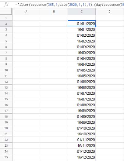
To generate bimonthly sequential dates likes 01-Jan-2020, 16-Jan-2020, 01-Feb-2020, 16-Feb-2020 and so on in a column or row in Google Sheets, we can use the SEQUENCE function with the FILTER function.
The above-said combination formula will populate the bimonthly dates in ascending order.
But if you want the bimonthly dates in descending order, I mean the dates in order like 01-Jan-2020, 16-Dec-2019, 01-Dece-2019 and so on, then we can use the SORT function additionally.
Also instead of 01 and 16, you can prefer any other bimonthly dates for example 7 and 23 like 07-Jan-2020, 23-Jan-2020, 07-Feb-2020, 23-Feb-2020 and so on. The formula is flexible enough for this change.
How to Get Bimonthly Dates in Ascending Order in Google Sheets
Bimonthly Dates in a Column (Asc)
Enter the below array formula in any blank column, for example in cell C2.
=filter(sequence(365,1,date(2020,1,1),1),(day(sequence(365,1,date(2020,1,1),1))=16)+(day(sequence(365,1,date(2020,1,1),1))=1))It will generate a list of date values. Select the date values (column C) and format it to dates from the format menu (Format > Number > Date).
The above array formula will generate the bimonthly sequential dates in Google Sheets from 01-Jan-2020 to 16-Dec-2020.

I will explain later how to edit this formula for different periods.
Bimonthly Dates in a Row (Asc)
Assume you want to create a Gantt chart template in Google Sheets.
You may have tasks start and end dates in two columns (B:C) and a row (D2:2) contains dates (daily, weekly, monthly, or fortnight bases) to draw the bar.

If the schedule is on a fortnight basis (in the above image it’s in weekly basis), then you may want to generate the bimonthly dates in a row.
In such a case, use TRANSPOSE with the above formula to get the output in a row.
=transpose(filter(sequence(365,1,date(2020,1,1),1),(day(sequence(365,1,date(2020,1,1),1))=16)+(day(sequence(365,1,date(2020,1,1),1))=1)))But if you know the SEQUENCE arguments, then you can avoid using TRANSPOSE by modifying the formula a little.
Syntax: SEQUENCE(rows, [columns], [start], [step])What you want to do is change the value used in ‘rows’ with ‘columns’ and the values used in ‘columns’ with ‘rows’. I mean replace 1 with 365 and 365 with 1 as below.
=filter(sequence(1,365,date(2020,1,1),1),(day(sequence(1,365,date(2020,1,1),1))=16)+(day(sequence(1,365,date(2020,1,1),1))=1))The above formula will generate bimonthly sequential dates in a row.
How to Modify the Formula?
Let me try to explain how to modify the formula to populate different bimonthly dates like;
- Different start and end month.
- Different dates (other two dates instead of 1 and 16).

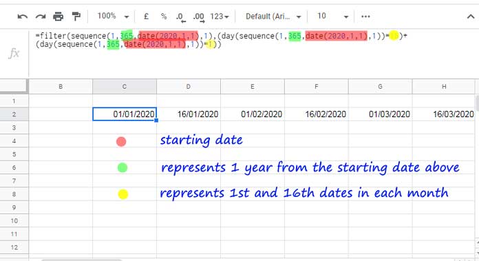
I think, with the help of the image, the formula seems easy for you to understand. Find more details below.
Legends and Explanation
Red Color: To get sequential bimonthly dates from 01-Jun-2020, change date(2020,1,1) which appears thrice in the formula with date(2020,6,1). The formula will return the dates from 01-Jun-2020 to 16-May-2021.
Green Color: Assume you have done the changes above (mentioned against red color). To get the dates only up to 16-Dec-2020 instead of 16-May-2021, you must change 365 in the formula with 213 that also thrice.
How I have come to this number?
Find the number of days (date difference) from 01-Jun-2020 to 31-Dec-2020 using the DAYS function below.
=days(date(2020,12,31),date(2020,6,1))Yellow Color: To get different bimonthly dates, replace 1 and 16 in the formula. For example, replace 1 and 16 with 7 and 23 and check the changes in the output
How to Get Bimonthly Dates in Descending Order in Google Sheets
Assume I want to get the dates from December 2020 to January 2020, that means dates in descending order. What we want to do is, use the start date as 01-Jan-2020 and 365 in the formula.
I mean use the same earlier formula. Then wrap it with SORT. How?
Generic Formula:
=sort(bimonthly_formula,1,0)So the formula will be;
In a Column:
=sort(filter(sequence(365,1,date(2020,1,1),1),(day(sequence(365,1,date(2020,1,1),1))=16)+(day(sequence(365,1,date(2020,1,1),1))=1)),1,0)In a Row:
We need to use the TRANSPOSE here as SORT won’t work in a row.
=transpose(sort(transpose(filter(sequence(1,365,date(2020,1,1),1),(day(sequence(1,365,date(2020,1,1),1))=16)+(day(sequence(1,365,date(2020,1,1),1))=1))),1,0))Formula Logic
To generate bimonthly sequential dates in Google Sheets I have used simple logic. It’s as follows.
The SEQUENCE formula generates sequential dates like 1-Jan-2020, 2-Jan-2020 and so on. The FILTER formula filters the dates 1 and 16.
Additional Resources
- How to Populate Sequential Dates Excluding Weekends in Google Sheets.
- Reset Week Number in Google Sheets Using Array or Non-Array Formulas.
- Calendar Week Formula in Google Sheets to Combine Week Start and End Dates.
- Weekday Name to Weekday Number in Google Sheets.
- How to Find Week Start Date and End Date in Google Sheets with Formula.
- How to Find Current Month’s Week Number In Google Sheets.
- Populate a Full Month’s Dates Based on a Drop-down in Google Sheets.
- How to Auto Populate Dates Between Two Given Dates in Google Sheets.
- Find the Past or Future Closest Date to Today in Google Sheets.
- Get a Dynamic Date that Advances/Resets in Google Sheets.
- How to Convert Date to Month and Year in Google Sheets.


