
The easiest way to convert a date to a month and year in Google Sheets is by using the TEXT function.
If your date is in cell A2, use this formula to get the full month and four-digit year (e.g., “January 2026”):
=TEXT(A2, "MMMM yyyy")If you need to apply this to an entire column at once without dragging it down, wrap it in an ARRAYFORMULA:
=ARRAYFORMULA(IF(ISBLANK(A2:A), "", TEXT(A2:A, "MMMM yyyy")))Common Month & Year Formats:
Depending on how you want your final result to look, simply replace "MMMM yyyy" in the formula with one of these patterns:
- Jan 2026:
"MMM yyyy" - January 2026:
"MMMM yyyy" - Jan-26:
"MMM-yy" - Jan ’26:
"MMM 'yy"(Note the single quote before yy) - 2026-01:
"yyyy-MM" - 01/2026:
"MM/yyyy"
3 Ways to Convert Dates to Month and Year in Google Sheets
While the TEXT function is the most popular way to change a date into a month and year, it isn’t the only option. If the TEXT function isn’t the right fit, you can get the same result using Custom Number Formatting or the QUERY function.
Each approach serves a different purpose depending on how you plan to use your data.
- Method 1: The TEXT Function – Best when you need a quick, text-based label in a separate column or want to use the result in text-matching formulas.
- Method 2: Custom Number Formatting – Best when you want to change how the date looks directly within its existing column without altering the underlying data.
- Method 3: The QUERY method is a little different. Instead of filtering or summarizing data, we’ll use its FORMAT clause to display dates as month and year while preserving the original date values.
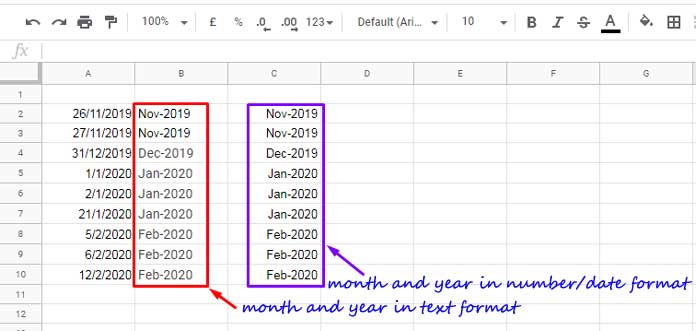
Method 1: The TEXT Function (For Text-Based Results)
Assume you have sales data entered in Google Sheets structured with columns for Date, Invoice, Customer, Product, and Amount.
If you want to find the total sales specifically for January 2026, you can use the TEXT function combined with SUMIF. Here is the formula:
=ARRAYFORMULA(SUMIF(IF(ISBLANK(A2:A), "", TEXT(A2:A, "MMMM yyyy")), "January 2026", E2:E))How This Formula Works
IF(ISBLANK(A2:A), "", TEXT(A2:A, "MMMM yyyy")): This converts the dates in column A into a text format of month and year (e.g., “January 2026”). TheIF(ISBLANK(...part ensures empty rows are ignored so they don’t incorrectly return “December 1899”.ARRAYFORMULA: This expands theTEXTandISBLANKfunctions so they process the entire column (A2:A) instead of just a single cell."January 2026": This is the matching criteria for yourSUMIF.E2:E: This is the sum range containing your sales amounts.
If you want to see this formula in action, copy my sample sheet by clicking the button below:
Method 2: Custom Number Formatting (Best for Preserving Date Values)
Assume you have the label Item in cell A1, and month start dates (e.g., 01/01/2026, 01/02/2026, 01/03/2026, …, 01/12/2026) laid out horizontally across cells B1:M1.
To convert these dates into a month and year format without altering the underlying date values, follow these steps:
- Select your date range:
Step 1.
Highlight the cells B1:M1 containing your dates. - Open the Custom Number Format settings:
Step 2.
In the top menu, click Format > Number > Custom number format. - Apply the format string:
Step 3.
Delete any existing placeholders in the text field at the top, typeMMMM yyyy, and click Apply.
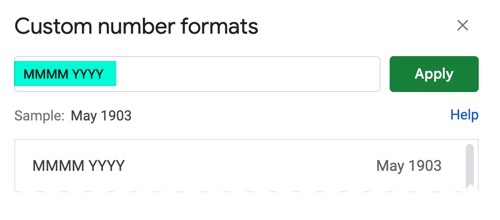
This will instantly display your dates as January 2026, February 2026, and so on. This is purely a visual mask. Feel free to use any of the alternative month and year format patterns we covered in the introduction to match your preferred style.
Method 3: The QUERY Function (Using the FORMAT Clause)
Let’s first look at how to use QUERY to convert a date to a month and year, and then we will look at a practical example.
The following formula masks the dates in range A2:A into a new column:
=QUERY(A2:A, "FORMAT Col1 ""MMMM yyyy"" ")Unlike the TEXT function, you do not need to wrap this in an ARRAYFORMULA here; the QUERY function handles the entire column automatically.
This formula purely applies a visual mask. To verify this, select any date in the query’s result and click Format > Number > Date—you will see that the underlying date value is still perfectly intact. You can use any of the month and year formatting variations specified in the introduction with this method.
Practical Example: Grouping Sales by Month
We usually do not use this method just to convert a single date column into a helper column. Instead, it becomes useful when you use it inside a query along with data grouping.
In this example, the sample data is in A1:E, with Sales Dates in column A, Items in column D, and Amounts in column E.
To summarize the data by month and item, follow these two steps:
Step 1: In cell F1, enter the following formula to create a helper column that normalizes all sales dates to month start dates:
=ARRAYFORMULA({"Month Start"; EOMONTH(A2:A, -1)+1})Pro Tip: On empty rows, EOMONTH with a second argument of -1 will simply return a #NUM! error. Do not use IFERROR to remove this error; doing so strips away the date formatting and converts the valid dates in your column into raw numbers (like 46023). Leaving the errors alone keeps your date formatting intact.
Step 2: Now, use this QUERY formula to generate your report:
=QUERY(A1:F, "SELECT Col6, Col4, SUM(Col5) WHERE Col4 IS NOT NULL GROUP BY Col6, Col4 FORMAT Col6 ""MMMM yyyy"" ", 1)How This Query Works
This query selects Column 6 (our new month-start helper column) and Column 4 (Item), sums up the 5th column (Amount), groups the totals by month and item, filters out any empty rows, and formats the final display to a clean month and year. Because the underlying data remains a true date (the first day of each month), your query output sorts chronologically.
Conclusion
Each method has its own purpose. Use TEXT when you need a month-year label, Custom Number Formatting when you only want to change the display, and QUERY when building grouped reports while preserving date values.
What’s Your Go-To Method?
Do you prefer the simplicity of the TEXT formula, or do you use the QUERY method for your reports? Let me know in the comments below!