Week numbers are a useful way to identify specific periods in a month or year. In this tutorial, you will learn how to calculate the Week Number Within Month for any given date in Google Sheets. To do this, we’ll use several built-in date functions.
The main functions we’ll use include WEEKNUM, TODAY, DATE, and EOMONTH. If you want a complete overview of date functions in Google Sheets, see my tutorial: How to Utilize Google Sheets Date Functions – Complete Guide.
Understanding the Concept with Examples
For example:
- If the date is 31/10/2013 (DD/MM/YYYY), it falls in Week 44 of the year and the fifth week of the month.
- For a past or future date, such as 15/03/2018, it falls in Week 11 of the year and Week 3 of March 2018.
While WEEKNUM can return the week of the year, calculating the Week Number Within Month requires a custom formula.
The WEEKNUM Function in Google Sheets
The WEEKNUM function returns the week number of the year in which a date falls.
Syntax:
WEEKNUM(date, [type])Arguments:
date: The date to determine the week number for.type(optional): Specifies the day the week starts on and the system used to determine the first week of the year (1 = Sunday, 2 = Monday).
Examples:
=WEEKNUM("15/03/2018")      // Returns 11
=WEEKNUM(DATE(2018, 3, 15))   // Returns 11
=WEEKNUM(A1)                // Returns 11 if A1 contains 15/03/2018
Note: By default, WEEKNUM considers Sunday to Saturday as one week. The week containing January 1 is the first week of the year.

Calculate Week Number Within Month in Google Sheets
Assume we have the date 15/03/2018 in cell A2. To find the Week Number Within Month for March 2018, use this formula:
=WEEKNUM(A2) - WEEKNUM(EOMONTH(A2, -1) + 1) + 1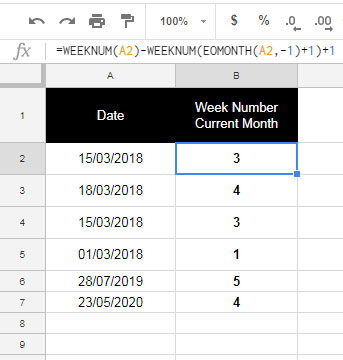
This formula returns 3, because March 15 falls in the third week of the month.
Week Ranges in the Month
For March 2018 (example for clarity):
| Week | Dates |
|---|---|
| 1 | Mar 1–3 |
| 2 | Mar 4–10 |
| 3 | Mar 11–17 |
| 4 | Mar 18–24 |
| 5 | Mar 25–31 |
Alternative Method:
If you prefer consecutive 7-day blocks starting from the 1st of the month (1–7 = Week 1, 8–14 = Week 2, etc.), you can use:
=ROUNDUP(DAY(A2)/7)How the Formula Works
The formula has two parts:
- Week Number of the Date:
=WEEKNUM(A2)This gives the week number of the year for the date in A2.
- Week Number of the Month Start:
=WEEKNUM(EOMONTH(A2, -1) + 1)EOMONTH(A2, -1)returns the last day of the previous month.- Adding
+1gives the first day of the current month.
Week Number Within Month Calculation:
Week Number Within Month = Week # of the Date - Week # of Month Start + 1Calculate Current Week Number Within Month
To find the current week of the month, replace the date with TODAY():
=WEEKNUM(TODAY()) - WEEKNUM(EOMONTH(TODAY(), -1) + 1) + 1Explanation:
TODAY()returns the current date.WEEKNUM(TODAY())gives the current week number of the year.WEEKNUM(EOMONTH(TODAY(), -1) + 1)gives the week number of the month’s first day.- Adding
+1ensures the first week of the month starts at 1.
You can also hardcode a specific date instead of TODAY() if needed, but using TODAY() makes your formula dynamic.
Conclusion
Calculating the Week Number Within Month (1–5) in Google Sheets is straightforward once you understand how the WEEKNUM and EOMONTH functions work together. By subtracting the week number of the month’s first day from the week number of your target date (and adding 1), you can accurately determine which week of the month any date belongs to.
This technique works both for historical and future dates, and with the TODAY() function you can dynamically track the current week of the month.
Related: How to Sum Data by Week of the Month in Google Sheets


Amazing job as usual, P. Thanks so much
Hi Prashanth,
Thanks for the correction. That works perfectly!
I have to admit, I’m not very familiar with the
LET()andLAMBDA()functions and only minorly familiar withMAP().Hi Prashanth,
I found this article when searching for help figuring out how many weeks in a month, contain a specific day (i.e. paychecks on Thursday). Your base formula was key to my solution so I thought I would post my solution here for anyone who might be looking to find the same thing.
While the
typeparameter ofWEEKDAY()is a straight-forward day offset from Sunday, thetypeparameter toWEEKNUM()is coded and is only available in the extended documentation. This threw me off initially.14is the correct value for `type` to use Thursday.The odd thing I found was that the
WEEKNUM()formula returned the incorrect number of weeks in a month, when the first of the month was on a Thursday. I thought for a while and couldn’t figure out how to alter the formula to correct that anomaly. Eventually I just decided to account for the edge-case.Here is my solution for finding the number of weeks in the month of a given date, contain a Thursday.
=WEEKNUM(EOMONTH(A1, 0), 14) -WEEKNUM(EOMONTH(A1, -1) + 1, 14) +
IF(WEEKDAY(DATE(YEAR(A1), MONTH(A1), 1)) = 5, 1, 0)
Hi Todd,
Thanks for sharing. Here is another way to handle this.
=COUNTIF(INDEX(WEEKDAY(SEQUENCE(DAY(EOMONTH(A1,0)),1,
EOMONTH(A1,-1)+1))),5
)
But you may require a Lambda to expand it, if necessary.
Hi Prashanth,
Interesting… I wasn’t able to get that to work inside an
ArrayFormula(), but I applied it manually against dates from 1/1/2020 -to- 12/1/2031 and it occasionally returned an extra week.I looked for a pattern that would expose the calculation error, but I couldn’t identify one. The following dates calculated 5 Thursdays instead of the 4 that exist in the month…
9/1/2020 (Tue) – 8 months later
6/1/2021 (Tue) – 9 months later
2/1/2022 (Tue) – 8 months later
11/1/2022 (Tue) – 9 months later
2/1/2023 (Wed) – 3 months later
4/1/2025 (Tue) – 26 months later
9/1/2026 (Tue) – 17 months later
6/1/2027 (Tue) – 9 months later
2/1/2028 (Tue) – 8 months later
2/1/2029 (Thu) – 12 months later
4/1/2031 (Tue) – 26 months later
Hi Todd,
That would work now! I made a mistake earlier, corrected that.
The logic is to generate a sequence for the whole month and count the weekdays equal to 5 in that sequence.
It’s flexible as you can replace 5 with any other weekday number.
You can follow this formula to make it an array formula:
=ARRAYFORMULA(LET(range, A1:A,
test,MAP(range,LAMBDA(row,COUNTIF(
WEEKDAY(SEQUENCE(DAY(EOMONTH(row,0)),1,EOMONTH(row,-1)+1)),5))),
IF(test=0,,test))
)
I think this breaks when the end of a week is also the end of the month.
So, assuming Sunday – Saturday weeks in March 2023.
The final day of the month is Friday. It is week 13 of 2023.
If I want the week number of April for April 7, 2023, the formula returns a two instead of a 1, although April 7 is in the first week (week 14).
Any ideas on how to work around that?
Hi, Parcoast,
Please follow the below steps to understand the formula.
We require three blank columns for the test.
1. Insert the following Sequence in cell A2 and then select A2:A > Format > Number > Custom Number Format >
dd"-"mmm"-"yyyy ddd=sequence(365,1,date(2023,1,1))2. In cell B2, insert the following Weeknum formula.
=ArrayFormula(weeknum(A2:A366,1))3. Finally, insert the following current month’s week number array formula in cell C2.
=ArrayFormula(WEEKNUM(A2:A366,1)-WEEKNUM((EOMONTH(A2:A366,-1)+1),1)+1)Go through every row and you will find the logic.
Also, check How to Sum by Week of the Month in Google Sheets.
Thanks a lot !
Hi Prashanth,
This still doesn’t quite work for me. For the month of May 2021, the results are still a week ahead. If I remove the last ‘+1’ and only have:
=WEEKNUM(A2,2)-WEEKNUM(EOMONTH(A2,-1)+1,2), then May is perfect, however, June then starts with Week 0.
Hi, Jamie,
The best way to understand my formula is as follows.
In a blank (new) Sheet, enter the following array formulas.
In Cell A2:
=sequence(35,1,date(2021,5,1))The formula would return a sequence of dates/date values from 1-May-2021 to 4-Jun-2021. Please select A2:A36 and apply Format (menu) > Number > Date.
In Cell B2:
=ArrayFormula(WEEKNUM(A2:A36)-WEEKNUM(EOMONTH(A2:A36,-1)+1)+1)The above is my array formula that returns the current month’s week number based on Sunday-Saturday weeks.
In Cell C2:
=ArrayFormula(WEEKNUM(A2:A36,2)-WEEKNUM(EOMONTH(A2:A36,-1)+1,2)+1)Your formula in Array Form (Monday-Sunday).
Now check the outputs.
Please don’t expect 7 full days in the first and the last week of the month as the formula considers Sunday-Saturday or Monday-Sunday to return the week numbers.
If you want 0-7 (1st week), 8-14 (2nd week), and so on as the week count basis, you can consider the below formula.
=roundup((days(A2,eomonth(A2,-1)+1)+1)/7)Thanks for this. However, it starts to fail in March/April of 2021. 29 March 2021 returns week#5 of March. However, the following Monday week (5 April 2021) returns as week#2 of April. Week#1 of April doesn’t exist!
Hi, Tedinoz,
The formula counts the week number of the entered date in that month NOT based on 1-7 (first week), 8-14 (second week), and so on. It is based on Sunday-Saturday.
Example:
1-May-2021 is Saturday which is week 1 in that month. Week 2 will be from 2-May-2021.
If you want the week to start from Monday-Sunday, modify the formula as below.
=WEEKNUM(A2,2)-WEEKNUM(EOMONTH(A2,-1)+1,2)+1Hope this clarifies.
This is so much helping!! Thanks a lot…
Thank you! Glad it helped.
Hello, I’m using a lot Google Sheets in my daily life and just want to say thank you for all the info, good practices, tricks you are publishing. It helps a lot!
Hi, Fabrice,
Thanks for taking time to leave your feedback!