Sum by the week of the month and by the week of the year is different. In this Google Sheets tutorial, we are discussing the former.
For this, first, we must know how to convert date to week number of month in Google Sheets.
If we consider the month of September 2022, once we convert the dates, there will be five months.
And for the conversion, we can choose different methods, and here we consider the below two.
| Week Nos. | Date Falls in Method 1 (Mon-Sun Week, which we can change) | Date Falls in Method 2 (doesn’t consider days of the week) |
| Week 1 | Thu, 01/9/22 – Sun, 04/9/22 | 01/9/22 – 07/9/22 |
| Week 2 | Mon, 05/9/22 – Sun, 11/9/22 | 08/9/22 – 14/9/22 |
| Week 3 | Mon, 12/9/22 – Sun, 18/9/22 | 15/9/22 – 21/9/22 |
| Week 4 | Mon, 19/9/22 – Sun, 25/9/22 | 22/9/22 – 28/9/22 |
| Week 5 | Mon, 26/9/22 – Fri, 30/9/22 | 29/9/22 – 30/9/22 |
| Week 1 | Sat, 01/10/22 – Sun, 2/10/22 | 1/10/22 – 7/10/22 |
As a side note, for sum by the week of the year, please check the following two tutorials.
- Summarize Data by Week Start and End Dates in Google Sheets.
- How to Create a Weekly Summary Report in Google Sheets.
Before creating the total by the week of the month, let’s go to the core.
How to Get Week of the Month in Google Sheets
We have a sample dataset in Google Sheets that contains the date and profit/loss of sale of goods in a trading company.
In the dataset, the range A2:A20 contain the dates and C2:C20 the profit/loss amount.
We will use these two columns to Sum by Week of the Month in Google Sheets.
First and foremost, we must know how to get the week of the month.
Method 1
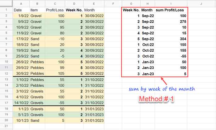
To get the week of the month as per method # 1, please use the following array formula in cell D1 after emptying D1:D.
(Please scroll down and see image # 1)
=ArrayFormula({"Week No.";if(A2:A="",,WEEKNUM(A2:A,2)-WEEKNUM(DATE(YEAR(A2:A),MONTH(A2:A),1),2)+1)})It will Reset Week Numbers when the month and also year changes.
You can also use the following alternative formula to get the week of the months as per method # 1.
=ArrayFormula({"Week No.";iferror(WEEKNUM(A2:A,2)-WEEKNUM(EOMONTH(A2:A,-1)+1,2)+1)})Related: How to Find Current Month’s Week Number In Google Sheets.
Both formulas follow the same logic, i.e.;
Week of the Month = week number of the date – week number of the month start of that date + 1
The vivid cyan part of the formula returns the date’s month start.
We have considered Monday-Sunday week by specifying type 2 (vivid red) in the formula.
To change that to Sunday-Saturday, please specify type 1 instead of 2.
Method 2
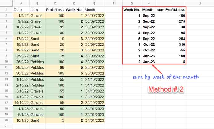
To get the week of the month as per method # 2, please use the following array formula in cell D1.
(Please scroll down and see image # 2)
=ArrayFormula({"Week No.";if(A2:A="",,roundup(day(A2:A)/7))})The formula divides day by seven days and rounds up that number. It’s that simple!
Sum by Week of the Month in Google Sheets
Whichever method you follow, the formula to sum by the week of the month is the same.
The output may vary depending on the D1 formula, which we have used to get the week of the month.
As mentioned, the sample dataset contains the date in A2:A and the profit/loss of sales in C2:C.
In E1, insert one more helper formula, which will return the end-of-the-month dates corresponding to the dates in A2:A.
=ArrayFormula({"Month";if(A2:A="",,eomonth(A2:A,0))})Must Check: How to Utilise Google Sheets Date Functions [Complete Guide]
Then check the returned values in E2:E. It may be date values instead of dates. If so, select E2:E and apply Format > Number > Date.
I’ll explain the importance of this formula later.
The following Query in G1 will return the total by the week of the month in Google Sheets.
=Query({A1:E},"Select Col4,Col5,sum(Col3) where Col4 is not null group by Col5,Col4 order by Col5 format Col5'mmm-yy'")Method # 1:

Method # 2:

What is the purpose of column E in the Query formula above?
If we group by column D (week of the month numbers), there will be an issue if you have dates spread across the months.
The same month numbers will be grouped even if they fall in two or more different months.
Column E acts as months in the formula.
We have chosen this column in Query to group the data along with column D.
With the help of the format clause, we have formatted column E to mmm-yy in the output instead of showing the end-of-the-months. But the underlying value will be the same end-of-the-months.
You May Like: Formula to Sort By Month Name in Google Sheets.
Sum by Week of the Month without Helper Columns
Our sales data is only in the range A1:C where column A contains dates, B items, and C profit/loss amount.
The rest of the columns used in the Query formula, i.e., D and E, act as two helper columns.
We can use them as virtual helper columns by modifying the Query data as below.
Current Data: {A1:E}
Replace it with the array {A1:C,D1_formula,E1_formula}
So the Sum by Week of the Month Query formula will become;
=Query({A1:C,ArrayFormula({"Week No.";iferror(WEEKNUM(A2:A,2)-WEEKNUM(EOMONTH(A2:A,-1)+1,2)+1)}),ArrayFormula({"Month";if(A2:A="",,eomonth(A2:A,0))})},"Select Col4,Col5,sum(Col3) where Col4 is not null group by Col5,Col4 order by Col5 format Col5'mmm-yy'")That’s all. Thanks for the stay. Enjoy!


