Learn how to summarize data by week start and end dates in Google Sheets — no helper columns needed. With just a transaction date column and an amount or quantity column, you can create a three-column summary showing the week start, week end, and total.
This guide includes three formulas: one for non-sequential week ranges, another for listing all weeks in sequence, and a third for custom week ranges based on your own date intervals.
Sample Data
We have sample data in the following structure in columns A and B:
| Date | Amount |
|---|---|
| 01/08/2020 | 5 |
| 02/08/2020 | 5 |
| 10/08/2020 | 5 |
| 14/08/2020 | 2 |
| 15/08/2020 | 2 |
| 16/08/2020 | 2 |
| … | … |
Let’s summarize this data by week start and end dates.
Summarize Data by Week Start and End Dates in Google Sheets (Only Weeks with Data)
In this approach, we include only the week ranges that have at least one date in column A. If a week range is missing because there are no transactions, it won’t appear in the summary. As a result, the week ranges may not be in sequence.
In the formula, we use data from the second row onward, skipping the header row since we add the headers manually in the formula.
Enter this formula in cell D1:
=ARRAYFORMULA(LET(
   wS, A2:A - WEEKDAY(A2:A, 2) + 1,
   wE, A2:A - WEEKDAY(A2:A, 2) + 7,
   amt, B2:B,
   data, HSTACK(wS, wE, amt),
   QUERY(data, "SELECT Col1, Col2, SUM(Col3) WHERE YEAR(Col1)<>1899 GROUP BY Col1, Col2 LABEL Col1 'Week Start', Col2 'Week End', SUM(Col3) 'Total'", 0)
))
This formula returns a summary based on a Monday–Sunday week.
To use a Sunday–Saturday week, replace 2 in the WEEKDAY function with 1.
Output:
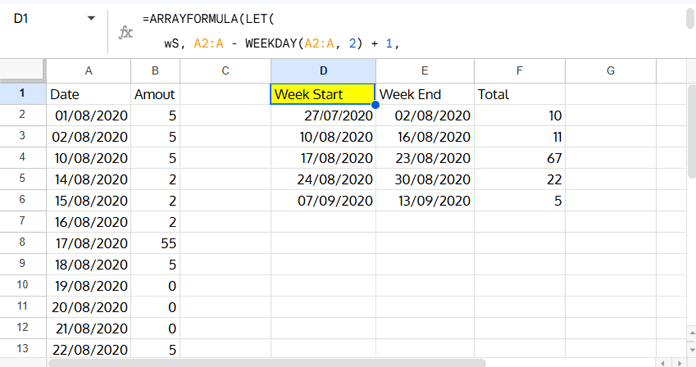
Note: If a week has at least one transaction but the total is 0, that week range will still be included. Empty weeks (no transactions) are excluded.
Formula Explanation
wS: Calculates the week start date by taking each date in column A and subtracting the weekday number (based on Monday = 2) minus 1. This aligns the date to the Monday of that week.wE: Calculates the week end date by adding 6 days towS(or by subtracting weekday and adding 7 directly).amt: Refers to the Amount column (B2:B).HSTACK(wS, wE, amt): Combines week start, week end, and amount into a single 3-column array.QUERY(...): Groups the data by week start and week end, sums the amounts, and labels the columns as “Week Start,” “Week End,” and “Total.”
The conditionWHERE YEAR(Col1)<>1899filters out rows created by blank/zero date values. Google Sheets treats an empty or zero date as a serial 0 date (December 30, 1899), and when the formula computes week start/end from that value it can produce a spurious week range such as 25/12/1899 – 31/12/1899. TheYEAR(Col1)<>1899check excludes those artifact rows.
Summarize Data by Week Start and End Dates in Google Sheets (All Weeks in Sequence)
If you want to list every week between the earliest and latest date in your data — including weeks where the total is 0 — use this formula:
Formula:
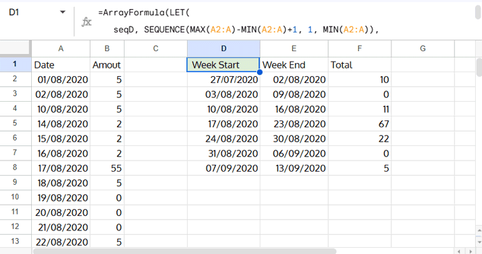
=ArrayFormula(LET(
   seqD, SEQUENCE(MAX(A2:A)-MIN(A2:A)+1, 1, MIN(A2:A)),
   wS, seqD-WEEKDAY(seqD, 2)+1,
   wE, seqD-WEEKDAY(seqD, 2)+7,
   amt, IFNA(VLOOKUP(seqD, QUERY(A2:B, "select Col1, sum(Col2) where Col1 is not null group by Col1 label sum(Col2) ''", 0), 2, FALSE), 0),
   data, HSTACK(seqD, wS, wE, amt),
   QUERY(data, "SELECT Col2, Col3, SUM(Col4) WHERE Col1 IS NOT NULL GROUP BY Col2, Col3 LABEL Col2' Week Start', Col3 'Week End', SUM(Col4) 'Total'", 0)
))
This formula returns the summary based on a Monday–Sunday week.
To change the start day, adjust the WEEKDAY function accordingly.
The Week Start and Week End columns in the result are date values.
Select those columns and go to Format → Number → Date to display them properly.
Output:
Formula Explanation
seqD
Generates a continuous list of dates from the earliest (MIN(A2:A)) to the latest (MAX(A2:A)) date in column A using SEQUENCE. This ensures that days with no transactions are still included.wSandwE
For each date inseqD, calculates the start (wS) and end (wE) dates of that week.WEEKDAY(seqD, 2)returns 1 for Monday, 7 for Sunday.- Subtracting this from the date and adding 1 gives the Monday of that week.
- Adding 7 gives the Sunday of that week.
amt
Uses a QUERY to group the original dataA2:Bby date and sum the amounts.- VLOOKUP then matches each date in
seqDto its daily total. IFNA(..., 0)replaces missing days with0so weeks with no data show as zero.
- VLOOKUP then matches each date in
data
CombinesseqD,wS,wE, andamtside-by-side using HSTACK.- Final
QUERY
Groupsdataby the week start and week end, summing the amounts for each week.
Labels are applied to make the output clear: Week Start, Week End, Total.
What If I Don’t Want to Follow the Calendar Week?
Sometimes you may want week ranges that don’t follow the standard calendar week. In that case, the first date in your data plus six days will be the first week, then the next seven days, and so on.
Formula for Week Ranges (Cell D2):
=LET(
   range, A2:A,
   n, (MAX(range) - MIN(range)) / 7,
   IFNA(
      HSTACK(
         SEQUENCE(n + 1, 1, MIN(range), 7),
         IFERROR(SEQUENCE(n, 1, MIN(range) + 6, 7), MAX(range))
      ),
      MAX(range)
   )
)
For a detailed explanation of how this formula works, see Convert Dates to Week Ranges in Google Sheets (Array Formula).
Formula for Totals (Cell F2):
=MAP(D2:D, E2:E, LAMBDA(wS, wE, IF(ISDATE(wS), SUMIFS(B2:B, A2:A, ">="&wS, A2:A, "<="&wE), )))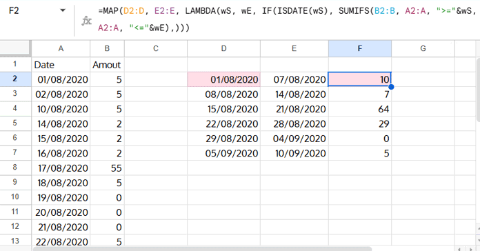
Formula Explanation
MAP(D2:D, E2:E, LAMBDA(...)): Loops through each week start (wS) and week end (wE).ISDATE(wS): Ensures only valid week start dates are processed.SUMIFS(...): Sums the values in column B where column A dates are between the current week start and week end (inclusive).- If
wSis not a valid date, returns blank.
This is another way to summarize data by week start and end dates in Google Sheets without sticking to calendar weeks.
Sample Sheet
You can get the sample sheet with all formulas entered below.
Resources
- Combine Week Start & End Dates with Calendar Week Formula
- Finding Week Start and End Dates in Google Sheets: Formulas
- Creating a Weekly Summary Report in Google Sheets
- How to Count Orders per Week in Google Sheets: Formula Examples
- How to Calculate Hours Worked Per Week in Google Sheets
- Conditional Week Wise Count in Google Sheets
- How to Sum by Week of the Month in Google Sheets
- How to Group by Week in Pivot Table in Google Sheets
- Sum Current Work Week Range with QUERY in Google Sheets
- Query Daily, Weekly, Monthly, Quarterly, and Yearly Reports in Google Sheets


I’m trying to summarize my data by week, but I want my Weekday to start on Friday and end on Thursday. So I can easily compare weekly income to weekly expenses. I know I can adjust the weekday start and end dates. But the sum column isn’t adjusting the totals to match the start and end dates.
Hi, Jesse,
I tested the formula and have found that the sum column is also adjusting. You may change all the
WEEKDAY(A2:A,2)toWEEKDAY(A2:A,15).In the formula that includes ‘Zero Transaction Weeks’, other than the above, you should change
WEEKDAY(sequence(days(max(A2:A),min(A2:A))+1,1,min(A2:A)),2)toWEEKDAY(sequence(days(max(A2:A),min(A2:A))+1,1,min(A2:A)),15)If you still have a problem, please share the URL of your SAMPLE sheet via comment, which I won’t publish.