In this quick Google Sheets tutorial, I will share the formula to convert month numbers to month names in Google Sheets. In addition, you can learn the following:

• How to convert a date to a month name.
• How to sort month names to month number order instead of alphabetical order.

Since the DATE function is used as part of the formula to convert month serial numbers to month names, it will convert any number to a month name. However, I have a fix to limit the numbers between 1 and 12. We will discuss more about this in the formula section below.

How to Convert Month Numbers to Month Names in Google Sheets

Suppose you have entered 1 in cell A1 in one of your Google Sheets spreadsheets. The following TEXT and DATE combination formula in cell B1 or any other blank cell can convert that month number to the corresponding month name, i.e., January.

=TEXT(DATE(2018,A1,1),"MMMM")

Enter 2 in cell A1 to get February, 3 to get March, 4 to get April, and so on.

The above formula would return the full name of the month. To get an abbreviated month name such as Jan, Feb, Mar, and so on, replace MMMM with MMM.

However, I do not recommend using this formula for converting month numbers to month names as it has an issue. Even if you feed it any numbers greater than 12 or less than 1, it will return month names. However, we want to limit it to 1 to 12. Before we do that, we must understand this formula.

Formula Logic

DATE function syntax: DATE(year, month, day)

We can use the DATE function to convert a provided year, month, and day into a date. We do not need to do anything with the day or year. Therefore, we can provide any day and year. The month number must be the number that we want to convert to a month name. We can enter it in any cell and refer to it as per our above formula, DATE(2018, A1, 1), or we can hardcode it, DATE(2018, 1, 1).

TEXT function syntax: TEXT(number, format)

We have used the TEXT function to format the date returned by the DATE function to a month name.

How to Limit Month Numbers to 1 to 12 in Google Sheets

One of the advantages of the DATE function is that it can add surplus months to years when converting the inputs. For example, the =DATE(2018, 24, 1) formula will return 01/12/2019.

So even if you provide any number in cell A1, such as 24, the earlier formula will convert it.

We do not have an issue with that or require it. However, if you want to limit month numbers to 1 to 12, you can use the ISBETWEEN function with the cell reference.

As per our first formula, to convert the month number in cell A1 to the corresponding month name in the text format, we can use the following formula:

=IF(ISBETWEEN(A1, 1, 12), TEXT(DATE(2018, A1, 1), "MMMM"), "")

Syntax of ISBETWEEN function:

ISBETWEEN(value_to_compare, lower_value, upper_value, [lower_value_is_inclusive], [upper_value_is_inclusive])

The above is the correct way to convert month numbers to month names in Google Sheets.

Array Formula to Convert Month Numbers to Month Names in Google Sheets

Sometimes we may have a cell range with month serial numbers from 1 to 12 and want to batch-convert them into month names in text.

We can easily convert our earlier formula. If the cell range is A1:A12, replace A1 in the earlier formula with A1:A12 and use the ARRAYFORMULA wrapper as follows.

=ARRAYFORMULA(IF(ISBETWEEN(A1:A12, 1, 12), TEXT(DATE(2018, A1:A12, 1), "MMMM"), ""))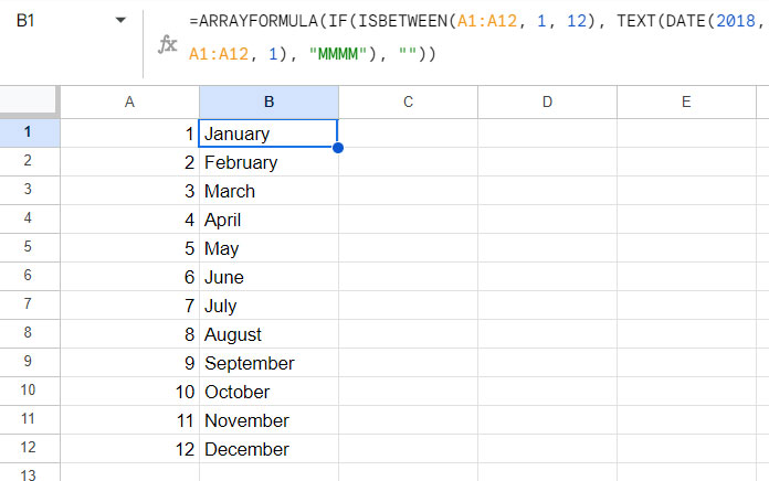

Do you want to get month names from January to December without referencing any range/array?

Replace A1:A12 with SEQUENCE(12) and here is that awesome formula.

=ARRAYFORMULA(IF(ISBETWEEN(SEQUENCE(12), 1, 12), TEXT(DATE(2018, SEQUENCE(12), 1), "MMMM"), ""))

How to Convert Date to Month Name in Google Sheets: Additional Tips

In the above examples, we have converted serial numbers from 1 to 12 to month names from January to December.

If you have a full date, meaning a valid date, instead of a serial number, you can convert it to a month’s name. There are three methods, two of which are formula-based and one is using a built-in menu command.

In the following examples, cell range A1:A12 contains valid dates. Here are the formulas that you can use to convert those dates to month names in text format.

QUERY Formula:

=QUERY(A1:A,"Select A where A is not null format A 'MMM'")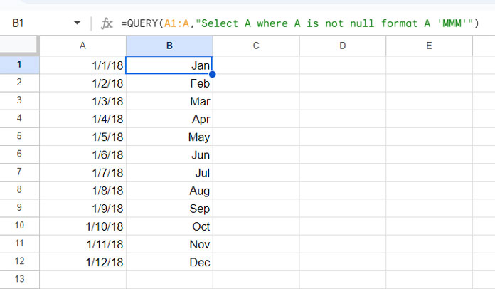

TEXT Formula:

=ARRAYFORMULA(IF(A1:A="",,TEXT(A1:A,"MMM")))

But some of you may want to make the change take effect in the same cell range, here A1:A12. In that case, we can use a menu command.

Here are those steps:

1. Select the date range to convert to the corresponding month names.
2. Go to the menu > Format > Number > Custom number format.
3. In the given field, either key in “MMMM” or “MMM” depending on whether you want full month names or abbreviated month names.
4. Click Apply.

Remember! The above two formulas and the menu command do not convert month numbers to month names. Instead, they require valid dates.

Sorting Month Names in Text to Month Number Order: Additional Tips

Here is yet another additional tip.

Sorting month names in proper month order can be tricky. This is because the Spreadsheet SORT function sorts texts in alphabetical order.

In column A, I have month names from January to December in unsorted form. I want it to be sorted month-wise, as shown in column D. How can I do this?

There are different ways to do this. Here, I will show you a method in which I will first convert the month name in text to the month number and then do the sorting.

=SORT(A1:A12,MONTH(A1:A12&1),TRUE)

If you want to learn this formula, please check my relevant tutorial here: Formula to Sort By Month Name in Google Sheets.

That’s all about converting month numbers to month names in Google Sheets.

Thanks for the stay. Enjoy!