Find the Closest Date to Today in Google Sheets

In order to find the closest date to today in Google Sheets, you can use the functions IF, TODAY, and MAX/MIN. The use of MAX, as well as the MIN function, depends whether you want to find the closest future date or closest past date.

Must Check: Vlookup Latest Date in Google Sheets

What’s the purpose of finding such dates? If you are a regular reader of my site, you may want to know the logic. If you have come to this post via a search engine, you know the purpose already.

Purpose:

Finding the future closest date to today is useful when you want to find the earliest date of shipment, availability of materials etc.

To find the last availability of an item which is not in stock, you can depend on the formula that finds the closest past date to today.

These are mere examples. You can find so many such instances in real life.

Formulas to Find the Closest Date to Today in Google Sheets

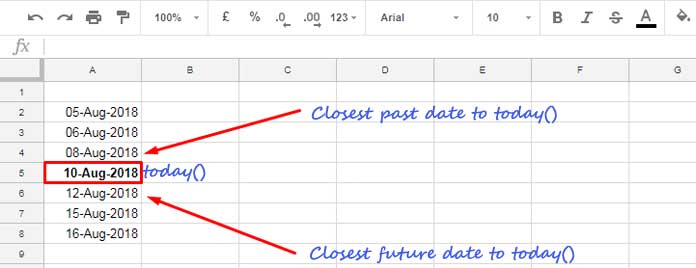
Today is 10th August 2018 as per my system clock. As per the list in column A, the closest past date to today is 08th August and the closest future date to today is 12th August.

Understand Closest Date to Today in Google Doc Sheets

In this, the dates are in chronological order. But your list of dates can be in sorted or unsorted order. The formulas that I am going to provide you are usable in any list irrespective of the order.

Here are the formulas to find the closest date to today in Google Sheets.

Find the Past Closest Date to Today

Formula:

=ArrayFormula(TO_DATE(MAX(if(A2:A<today(),A2:A))))

In this formula the To_date is optional.

What is the logic? With the IF logical test, we can find the dates that are< today. The MAX function returns the latest date from that output and that would be the past date closest to today.

Find the Future Closest Date to Today

Formula:

=ArrayFormula(TO_DATE(MIN(if(A2:A>today(),A2:A))))

Here the IF formula finds the dates that are> today. The MIN function returns the earliest date from the output and that would be the future closest date to today.

Can you explain to me why you have used the To_date function in these two formulas?

The To_date function formats a date value to date. Without this, you may have seen a date value as output instead of date. So the solution is either format the cell to date from the format menu or use the To_date function to bring back the date value to date.

I have used the ARRAYFORMULA as the IF is used in an Array, not in a single cell.

Additional Tips: Closest Date to Today in Vlookup

You have learned how to find the closest date to today() in Google Sheets. It can be past date or future date. Do you know how to use this in Vlookup?

See this example.

Vlookup to Lookup Closest Date to Today

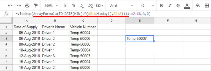
In this Vlookup, I have used one of my above formula (which is underlined in red color) that finds the closest future date to today as the search_key.

VLOOKUP(search_key, range, index, [is_sorted])

The range is the actual data range A2: C8 and I want the value from 3rd column (index).

That means we can use my formulas above to lookup closest date to today in Google Sheets Vlookup formula to find the required information from the corresponding cell/cells in the row.

Note: The formula that you can see in the screenshot has to be modified as below.

=ArrayFormula(vlookup(TO_DATE(MIN(if(A2:A>today(),A2:A))),A2:C8,3,0))

In this, I’ve moved the ArrayFormula to the first. But both the formulas will work without any issue.

That’s all. Enjoy!

27 COMMENTS

Andy May 10, 2023 At 5:49 pm

Hi,

Is there a way to look up the next date to today from a list of dates in another workbook, please?

Thank you.

- Prashanth May 11, 2023 At 2:47 pm
  
  Hi, Andy,
  
  Import the data and use one of my above formulas.
  
  To import, use the IMPORTRANGE function.
  
Jeffrey January 5, 2023 At 1:15 am

Thank you so much for your answer.

I am using this formula to see my clients’ birthdays, and sometimes I have multiple clients that have their birthdays on the same day.

How can I have the formula post all the results if there are multiple of the same date?

Also, is there a way to filter this to see all upcoming birthdays within the next day or week?

Thank you so much.

- Prashanth January 8, 2023 At 11:06 am
  
  Hi, Jeffrey,
  
  Use FILTER to filter the table.
  
  For example, if the dates are in A2:A and client names in B2:B, you can use the below formula.
  
  =filter(A2:B,A2:A=TO_DATE(MAX(if(lt(A2:A,today()),A2:A))))
  
CG September 9, 2022 At 10:58 pm

Can you help me: what would the formula be if I wanted to find the 2nd next future date among a set of dates?

- Prashanth September 10, 2022 At 9:50 am
  
  Hi, CG,
  
  This may help.
  
  =ArrayFormula(to_date(iferror(small(if(A2:A>today(),A2:A),2))))
  
Dom September 8, 2022 At 7:28 am

Hi Prashanth,

Thank you for posting this solution to finding the closest date as well as a value related to it.

I had a few bumps when implementing that I was hoping you could help with.

1. The formula returned an error when the date column wasn’t the first column.

2. How would you handle the situation when multiple occurrences happen on the same upcoming date?

Thanks!

- Prashanth September 10, 2022 At 9:42 am
  
  Hi, Dom,
  
  Q1 (Answer):
  
  I understand that the date column is not the first column. Since Vlookup searches the first column, you require to re-structure the column virtually.
  
  In my Vlookup formula, the source range is A2:C8, where A2:A8 contain dates.
  
  If B2:B8 contain dates insted, you can re-arrange it as {B2:B8,A2:A8,C2:C8}
  
  So the formula will become
  
  =ArrayFormula(vlookup(TO_DATE(MIN(if(B2:B8>today(),B2:B8))),{B2:B8,A2:A8,C2:C8},3,0))
  
  Please check the details under the subtitle “Leftward Vlookup – Vlookup Advanced Tips # 4” in the Vlookup function guide.
  
  Q2 (Answer):
  
  Multiple occurrences in Vlookup is a different topic. You can read that here.
  
sruli March 28, 2022 At 6:12 pm

Prashanth,

Regarding my last message (not yet published) you can ignore, I found 1 of the cells in my date list had =TODAY() 😉

- Prashanth March 29, 2022 At 10:53 am
  
  Hi, truly,
  
  I’ve read that comment.
  
  It seems the ‘working’ formula that you have shared in that, itself, was not correct.
  
  Please feel free to share the URL of your (sample) sheet in the below reply. I won’t publish.
  
Spencer February 19, 2022 At 7:14 am

Hi, Prashanth,

Do you have any idea why conditional formatting is not being applied to a column with dates in it generated by a REGEXEXTRACT formula?

It works for a random date I entered in Column C, but not for dates in Column B.

Formula:

={"Exp Date Only";arrayformula(if(A2:A="",,REGEXEXTRACT(A2:A,"[0-9]{2}/[0-9]{2}/[0-9]{4}")))}

Thanks for your help!

- Prashanth February 20, 2022 At 3:42 pm
  
  Hi, Spencer,
  
  The output is text. Use the VALUE function around your Regex.
  
  E.g.:-
  
  ={"Exp Date Only";arrayformula(if(A2:A="",,value(REGEXEXTRACT(A2:A,"[0-9]{2}/[0-9]{2}/[0-9]{4}"))))}
  
  An alternative Regex formula.
  
  ={"Exp Date Only";arrayformula(if(A2:A="",,value(REGEXEXTRACT(A2:A,"[0-9/]+"))))}
  
  When you use this, you must format the output to Date from the Format menu.
  
Mina Boulos January 19, 2022 At 3:03 am

Hello, I would like to know how to adapt this formula to two VLOOKUPs instead of only the date.

I want the date and another normal VLOOKUP criterion. Thanks.

- Prashanth January 19, 2022 At 9:24 am
  
  Hi, Mina Boulos,
  
  There are many options. Here is one.
  
  Note:- The following examples are as per the table below the subtitle “Additional Tips: Closest Date to Today in Vlookup.”
  
  Past:
  
  =sortn(filter(A2:C,lt(A2:A,today()),B2:B="Driver 2"),1,0,1,0)
  
  Future:
  
  =sortn(filter(A2:C,gt(A2:A,today()),B2:B="Driver 2"),1,0,1,1)
  
  The above formulas will return all the columns. Wrap it with Query to select required columns.
  
  E.g.:-
  
  =query(sortn(filter(A2:C,lt(A2:A,today()),B2:B="Driver 2"),1,0,1,0),"Select Col2,Col3")
  
Alex January 29, 2021 At 5:11 am

Hi, is there a version of this that doesn’t use TODAY? But uses a specific date? eg: 12/1/20. I’ve tried multiple versions using a specific date, but it mostly returns 0.

- Alex January 29, 2021 At 5:13 am
  
  NM, I immediately figured it out after I posted this. Subbed TODAY() for DATE(2020,12,01) and it worked.
  
- Heidi January 4, 2022 At 11:49 pm
  
  Were you able to ever figure out a way to have it lookup against a specific date that is a referenced date vs. a hard-coded date?
  
  - Prashanth January 5, 2022 At 11:40 am
    
    Hi, Heidi,
    
    Enter the hard-coded date using the DATE() function.
    
    Date to lookup: 31/12/2021
    Referenced date: D2
    Hard-coded date:=date(2021,12,31)
    
Abbe December 9, 2020 At 7:29 pm

Thank you for the valuable tutorial!

Is there’s a way to implement this logic to find the closest TIME to the current time?

I have a list of dates (DATETIME) and some may fall on the same day but at different times.

Please provide guidance if this’s possible!

Thank you in advance!

- Prashanth December 10, 2020 At 6:03 am
  
  Hi, Abbe,
  
  Replace today() in the formulas with now().
  
  If the result shows only date, format the result to timestamp from the menu Format > Number > Date time.
  
  - Abbe December 11, 2020 At 7:36 pm
    
    Thank you for your quick and helpful reply!
    Using now() did the trick.
    
sruli s September 9, 2020 At 10:02 pm

Thank you very much for the formula, I have an issue I hope you can tell me how to resolve it.

If I use the formula to get the closest date in the future and the range only has past dates I get a result ‘Dec,30,1899’ what do I need to add so the result should be blank if there is no future date?

Many thanks.

- Prashanth September 10, 2020 At 9:44 am
  
  Hi, sruli s,
  
  Thanks for letting me know about the issue. Actually the said date “Dec,30,1899” is equal to 0. The To_Date in the formula converts 0 to “Dec,30,1899”.
  
  You can solve the issue and RETURN BLANK IF NO SATISFYING DATE by using the below formulas.
  
  I am using Maxifs and Minifs this time though the Max+If and Min+If will also work.
  
  Maxifs formula to find the past closest date to today():
  
  =if(maxifs(A2:A,A2:A,"<"&today())>0,to_date(maxifs(A2:A,A2:A,"<"&today())),"")
  
  Minifs formula to find the future closest date to today():
  
  =if(minifs(A2:A,A2:A,">"&today())>0,to_date(minifs(A2:A,A2:A,">"&today())),"")
  
  I hope these formulas help?
  
Matthew August 19, 2020 At 5:28 pm

Hi, is there a way to adapt this formula for several columns of dates?

- Prashanth August 21, 2020 At 9:23 am
  
  Hi, Matthew,
  
  Yup! Assume the dates are in columns A, B, and C.
  
  To find the past closest date, you can use the below formula.
  
  =ArrayFormula(TO_DATE(MAX(if(lt(A1:C,today()),A:C))))
  
  Here is a new formula using FLATTEN and FILTER (just for learning more)
  
  =to_date(sortn(filter(flatten(A1:C),lt(flatten(A1:C),today())),1,2,1,0))
  
  Similarly, to return the future closest date to today() in multiple columns, use either of the following two formulas.
  
  =ArrayFormula(TO_DATE(MIN(if(gt(A1:C,today()),A:C))))
  
  Here is the FLATTEN one.
  
  =to_date(sortn(filter(flatten(A1:C),gt(flatten(A1:C),today())),1,2,1,1))
  
  See if this helps?
  
Eran Chazan June 19, 2020 At 11:22 am

I need to Find the Past Closest Date to Today but for a specific landowner.

That is I need to add a second IF statement inside the array_formula that pulls from column B where B = ‘land_owner_name’
to: =ArrayFormula(TO_DATE(MAX(if(Com_Log!A:A<today(),Com_Log!A:A))))

Can this be done?

- Prashanth June 19, 2020 At 6:41 pm
  
  Hi, Eran Chazan,
  
  Your question is how to find the past closest date to today() with a condition included.
  
  You may try to use the below formula. In that instead of IF + MAX, I’ve used MAXIFS as multiple max conditions are involved.
  
  =to_date(MAXIFS(A2:A,A2:A,"<"&today(),B2:B,"james"))
  
  Replace "james" with the landowner name.