We can use the TEXT, SEQUENCE, and XLOOKUP functions to convert weekday names (days of the week) into numbers in Google Sheets.
Why should you learn this technique?
If you have weekday names in a table and you want to sort it, it will sort alphabetically, not by the order of weekdays.
Knowing how to convert weekday names to numbers will be useful, as you can use the numerical representation as the ‘sort by’ column.
Related: Sort by Day of the Week in Google Sheets.
Another use case is charting. Numeric values are often more suitable for creating charts, making it easier to represent and interpret patterns in data over weekdays.
Assume you have day-of-the-week strings in a column from Sunday to Saturday or Sun to Sat.
How would you return the corresponding day-of-the-week numbers in another column using array or non-array formulas?
You can use many combinations of formulas, but we will follow a unique approach that utilizes the TEXT, SEQUENCE, and XLOOKUP combo.
How to Convert Weekday Names to Numbers in Google Sheets
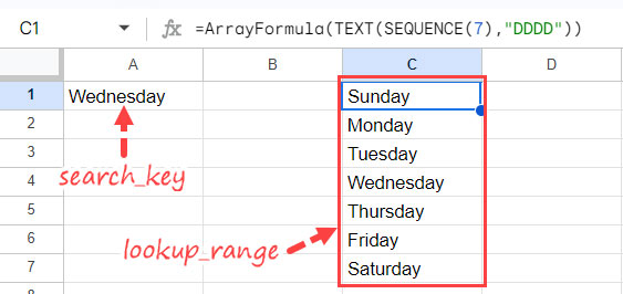
We will use XLOOKUP to look up the search keys (search_key), in this case, the weekday names, in one array (lookup_range) and return the corresponding numbers from another array (result_range).
Syntax:
XLOOKUP(search_key, lookup_range, result_range, [missing_value], [match_mode], [search_mode])Note: The optional arguments within square brackets are not required for this type of lookup operation.
The first array will contain the weekday names, and the second will contain the corresponding numbers.
What makes the formula interesting is the way we generate these two arrays. We will use the TEXT and SEQUENCE combination for the first array and SEQUENCE for the second array.
Let’s delve into these tips and convert weekday names to numbers.
Steps
Step 1: Search Key
It is up to you whether you want to convert several weekday names to corresponding numbers in one go or one by one. We will start with one value in cell A1 and then use the formula to convert A1:A or any range you prefer.
For example, suppose the search key is “Wednesday” in cell A1.
Step 2: Generating the Lookup Range
In one of my earlier tutorials titled “How to Autofill Days of the Week in Google Sheets,” I’ve shown two methods to autofill weekday names in a column. The first method uses a built-in non-formula approach, and the second method uses an array formula. We will use that array formula to generate the lookup range.
=ArrayFormula(TEXT(SEQUENCE(7), "DDDD"))For the time being, input this formula in cell C1.
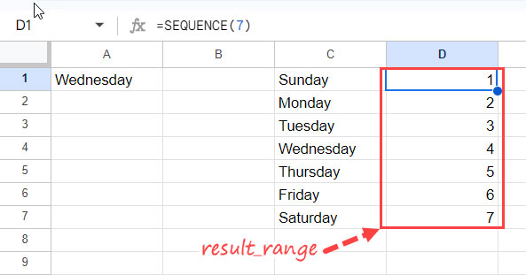
Step 3: Generating the Result Range
The resulting range is simply sequence numbers 1 to 7. We will use the following SEQUENCE function.
=SEQUENCE(7)For the time being, input this formula in cell D1.
Formula to Convert Weekday Names to Numbers:
To convert the weekday name in cell A1 to the corresponding weekday number, use the following formula in cell B1.
=XLOOKUP(
    A1,
    ArrayFormula(TEXT(SEQUENCE(7),"DDDD")),
    SEQUENCE(7),
)
Where:
A1is thesearch_key.ArrayFormula(TEXT(SEQUENCE(7),"DDDD"))is thelookup_range.SEQUENCE(7)is theresult_range.
But wait. As a standard practice, let’s move the ArrayFormula function to the beginning of the formula:
Final Formula:
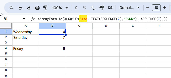
=ArrayFormula(XLOOKUP(
    A1,
    TEXT(SEQUENCE(7),"DDDD"),
    SEQUENCE(7),
))
To convert the weekday names in column A (A1:A), you may replace the search key A1 with A1:A. That’s it.
Additional Tips
1. Managing Abbreviations of Weekday Names in the Search Key Column
When converting weekday names to numbers, it’s crucial to account for one thing. The previous formula isn’t configured to handle abbreviated weekday names such as “Sun” for “Sunday.”
If you have abbreviated weekday names, modify the formula by replacing the text formatting style "DDDD" with "DDD":
=ArrayFormula(XLOOKUP(
    A1:A,
    TEXT(SEQUENCE(7), "DDD"),
    SEQUENCE(7),
))
If your data includes both abbreviated and non-abbreviated forms of weekday names, you can use the following formula:
=ArrayFormula(XLOOKUP(
    A1:A,
    VSTACK(TEXT(SEQUENCE(7), "DDDD"), TEXT(SEQUENCE(7), "DDD")),
    VSTACK(SEQUENCE(7), SEQUENCE(7)),
))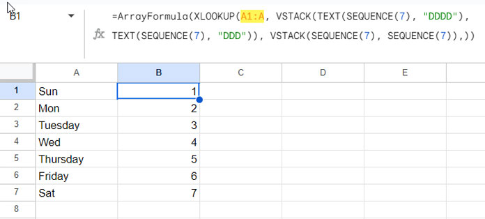
This formula is versatile, capable of handling abbreviated, non-abbreviated, and a mix of both weekday names.
The VSTACK function is employed to vertically stack both types of weekday names in the lookup range and appropriately stack the numbers.
2. Converting Weekday Names to Numbers with Custom WEEKDAY Types (e.g., 1 for Monday, 7 for Sunday)
The WEEKDAY function, one of the date functions, in Google Sheets assists in extracting weekday numbers from dates.
As you may know, we have the option to obtain weekday numbers 1-7 for Sunday-Saturday or 1-7 for Monday-Sunday by specifying the ‘type’ in this function.
Our above formulas, designed to convert weekday names (not dates) to numbers, are coded to return 1-7 for Sunday- Saturday. In most cases, such as for sorting and charting, this may be sufficient.
But if you want to alter that and get 1-7 for Monday- Sunday, you can easily achieve that by modifying the SEQUENCE formula part in the lookup range.
The current formula part is SEQUENCE(7). You need to modify it to SEQUENCE(7, 1, 2).
So the formula will be:
=ArrayFormula(XLOOKUP(
    A1:A,
    TEXT(SEQUENCE(7, 1, 2), "DDDD"),
    SEQUENCE(7),
))
Replace “DDDD” with “DDD” based on whether you have non-abbreviated or abbreviated weekday names.
If you prefer the all-weather formula, it would be as follows:
=ArrayFormula(XLOOKUP(
    A1:A,
    VSTACK(TEXT(SEQUENCE(7, 1, 2), "DDDD"), TEXT(SEQUENCE(7, 1, 2), "DDD")),
    VSTACK(SEQUENCE(7), SEQUENCE(7)),
))
With this, we conclude this tutorial. We welcome your suggestions and feedback.


