How to Fill Missing Dates in Google Sheets (Categorized & General)

We will approach the task of filling in missing dates in Google Sheets more broadly, whether with or without a category column. We will use two separate formulas for each task.

The formulas are complex, but there is no need to worry about their implementation. Your sole task is to accurately specify the range references in the formula, and they appear only once in the formula.

You can utilize the formulas for two types of data sets: one with a date and amount column (general), and the other with a category, date, and amount column (categorized).

A notable feature of these formulas is their array functionality, efficiently filling in missing dates and generating the table in one go. There is no need for helper columns or dragging down the formula.

Another advantage is their ability to retain values without merging when there are multiple occurrences of a date for a single transaction.

If you’re curious about potential drawbacks, there are two to consider.

Firstly, they utilize lambda helper functions, which may experience slowdowns or cease functioning in large datasets.

Secondly, it might pose a challenge for beginners to comprehend. However, understanding the logic behind the formulas is not necessary, as you can use them without delving into their intricacies. Nevertheless, I will explain how the formulas fill in missing dates for those interested in the details.

Filling Missing Dates in Google Sheets: General Method

In this approach, we will use two columns: a date column and another column with amounts or any values.

Key in the following formula in cell E2 to fill in missing dates in the data range B2:C100, where B2:B100 contains dates, and C2:C100 contains amounts (C2:C100 can be any values). In the formula, you just need to specify the date column reference.

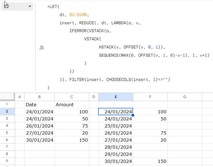
Filling Missing Dates in Google Sheets Using the Two-Column Approach

Formula 1:

=LET(
     dt, B2:B100, 
     insert, REDUCE(, dt, LAMBDA(a, v, 
         IFERROR(VSTACK(a, 
               VSTACK(
                     HSTACK(v, OFFSET(v, 0, 1)), 
                     SEQUENCE(MAX(0, OFFSET(v, 1, 0)-v-1), 1, v+1)
               )
         ))
     )), FILTER(insert, CHOOSECOLS(insert, 1)<>"")
)

Important:

The range B2:C100 must be sorted with the date column in ascending order.

After applying the formula, ensure proper formatting for the dates column in the result. Select the date values in the result and apply Format > Number > Date.

Formula 1 Breakdown:

The formula utilizes the LET function to assign names to ranges/expressions.

Syntax:

LET(name1, value_expression1, [name2, …], [value_expression2, …], formula_expression)

Defined Names and Value Expressions:

name1: dt
- value_expression1: B2:B100 (the date range)

name2: insert
- value_expression2:

REDUCE(, dt, LAMBDA(a, v,
   IFERROR(VSTACK(a,
      VSTACK(
         HSTACK(v, OFFSET(v, 0, 1)),
         SEQUENCE(MAX(0, OFFSET(v, 1, 0) - v - 1), 1, v + 1)
      )
   ))
))

This value_expression2 is a crucial part of the formula that fills in missing dates in the two-column table.

It employs a REDUCE function, iterating through each value in the date column and executing a lambda function. The key part of the lambda function is as follows:

VSTACK(
   HSTACK(v, OFFSET(v, 0, 1)),
   SEQUENCE(MAX(0, OFFSET(v, 1, 0) - v - 1), 1, v + 1)
)

It vertically stacks the current element (‘v’) and the value in the next column with sequence dates.

The SEQUENCE part returns n sequence values if the current next element value – current element value – 1 is greater than 0, with the sequence starting from the current element + 1. This process repeats in each row of the date range.

To get the accumulated result, VSTACK(a, …) is used before the key part. The IFERROR function removes any potential errors due to stacking mismatching arrays and sequence errors.

Formula Expression:

FILTER(insert, CHOOSECOLS(insert, 1)<>"")

This expression filters out blank rows from the first column of “insert.”

Follow this approach when you don’t want to fill in missing dates categorized.

Filling Missing Dates in Google Sheets: Category-Based Approach

For this approach, we are dealing with a three-column table: Category, Date, and Amount.

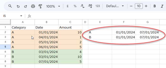
What adds complexity to the challenge is the presence of a category column in the table. Let’s assume we have two categories.

The minimum and maximum dates for the first category are 01/01/2024 and 06/01/2024, respectively, and for the second category, they are 03/01/2024 and 07/01/2024.

After applying the formula, it is expected that each category will have an equal number of records. Consequently, the start and end dates for both categories should be adjusted to 01/01/2024 and 07/01/2024.

Handling missing dates becomes challenging in this scenario. Here is how to address this in Google Sheets.

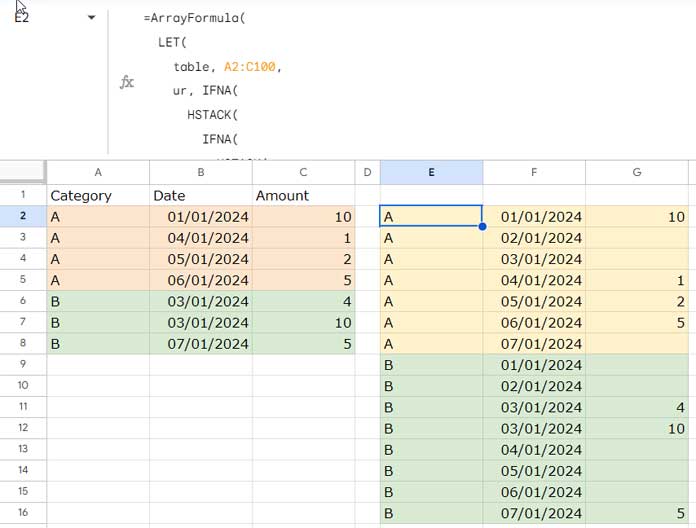
Filling Missing Dates by Category in Google Sheets Using the Three-Column Approach

Formula 2:

=ArrayFormula(
  LET(
    table, A2:C100, 
    ur, IFNA(
      HSTACK(
        IFNA(
          HSTACK(
            TOCOL(UNIQUE(CHOOSECOLS(table, 1)), 3), 
            MIN(CHOOSECOLS(table, 2))
          ), MIN(CHOOSECOLS(table, 2))
        ), MAX(CHOOSECOLS(table, 2))
      ), MAX(CHOOSECOLS(table, 2))), 
    seq, MAP(
      CHOOSECOLS(ur, 1), CHOOSECOLS(ur, 2), CHOOSECOLS(ur, 3), 
      LAMBDA(x, y, z, 
        LET(
          test, SEQUENCE(1, z-y+1, y), 
          FILTER(
            test, 
            IFNA(XMATCH(x&test, CHOOSECOLS(table, 1)&CHOOSECOLS(table, 2)))=""
          )
        )
      )
    ), 
    missing, HSTACK(TOCOL(IF(seq, CHOOSECOLS(ur, 1),)), TOCOL(seq)), 
    IFNA(SORT(VSTACK(table, missing), 1, 1, 2, 1))
  )
)

Important:

The range A2:C100 must be sorted by column A (category) in ascending order, and then by column B (date) in ascending order.

After applying the formula, ensure proper formatting for the date values in the result. Select the date values and apply Format > Number > Date.

Formula 2 Breakdown:

Let’s see how the formula fills in missing dates categorized in Google Sheets.

Here also, we have used the LET function to simplify the formula. Below are the defined names, value expressions, and the formula expression explained in detail.

Defined Names and Value Expressions:

name1: table
- value_expression1: A2:C100 (the table range)

name2: ur
- value_expression2:

IFNA(
  HSTACK(
    IFNA(
      HSTACK(
        TOCOL(UNIQUE(CHOOSECOLS(table, 1)), 3),
        MIN(CHOOSECOLS(table, 2))
      ), MIN(CHOOSECOLS(table, 2))
    ), MAX(CHOOSECOLS(table, 2))
  ), MAX(CHOOSECOLS(table, 2))
)

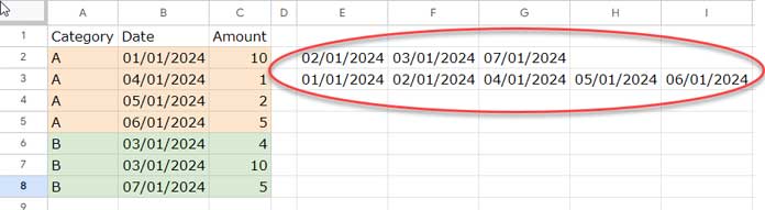
The ‘ur’ part extracts unique categories and horizontally stacks them with a common minimum start date in one column and a common maximum date in another column.

It returns a three-column table with unique categories, common minimum start dates, and common maximum end dates. The UNIQUE, IFNA, VSTACK, and HSTACK functions are employed for this purpose.

Display of Unique Categories with Common Min and Max Start and End Dates

name3: seq
- value_expression3:

MAP(
  CHOOSECOLS(ur, 1), CHOOSECOLS(ur, 2), CHOOSECOLS(ur, 3),
  LAMBDA(x, y, z,
    LET(
      test, SEQUENCE(1, z-y+1, y),
      FILTER(
        test,
        IFNA(XMATCH(x&test, CHOOSECOLS(table, 1)&CHOOSECOLS(table, 2)))=""
      )
    )
  )
)

We use the MAP lambda function to iterate over each value in the three-column ‘ur’ table, expanding start and end dates in each row, and filtering out dates category-wise that already exist in the ‘table’.

Expanded View of Missing Dates (Before Combining with Source Table)

name4: missing
- value_expression4:

HSTACK(TOCOL(IF(seq, CHOOSECOLS(ur, 1),)), TOCOL(seq))

The IF logical test returns the category in each row corresponding to the expanded dates. The TOCOL function makes it a single column. With this, we horizontally stack the expanded dates after making it a column.

Formula Expression:

IFNA(SORT(VSTACK(table, missing), 1, 1, 2, 1))

Combine the missing dates with the original table, sorting it by column 1 (category) in ascending order, and then by column 2 (date) in ascending order.

How Filling Missing Dates in a Table is Useful in Google Sheets

Filling missing dates in a table has several advantages in data manipulation and visualization. This approach proves especially useful in charting and running totals.

Filling in missing dates ensures that your data is continuous, creating smoother line charts that accurately represent trends over time. Additionally, having a complete set of sequential dates ensures a consistent X-axis, providing a clearer representation of time-based data.

For scenarios where you need running counts or cumulative totals over time, having a complete set of dates allows for accurate calculations without gaps.

We have already implemented running total array formulas that involve category-wise running totals as well. You can use them once you insert missing dates in your table.

Resources

This tutorial describes two approaches to filling in missing dates in a table. The following tutorials discuss advanced data manipulation techniques involving dates and date ranges.