To duplicate rows based on start and end dates in Google Sheets, we will employ the REDUCE function as a key tool. Its logic aligns with that of filling in missing dates.
The main advantage of this REDUCE method lies in its array functionality, eliminating the need for helper cells, columns, or rows.
However, a drawback to consider before using it is that the REDUCE function may result in a slowdown in performance or may cease to function altogether with large volumes of data.
Keep this limitation in mind when automating row duplication based on start and end dates in Google Sheets.
Duplicating Rows Based on Start and End Dates in Google Sheets
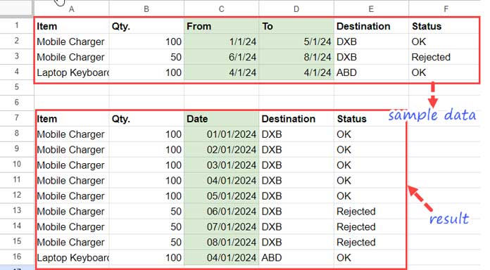
For testing purposes, we’ll use sample data within the range A1:F4 as follows (A1:F1 contains the field labels).
This data includes columns for Item, Qty., From, To, Destination, and Status, found in columns A, B, C, D, E, and F, respectively. In essence, it represents the status of material supply.
First, let’s delve into the formula and understand how to adapt it to your table with a different layout. Subsequently, we’ll proceed to the intriguing formula explanation part.
=ArrayFormula(REDUCE(
     TOCOL(,1), C2:C4, LAMBDA(a, v,
          VSTACK(a,
               LET(
                    seq, SEQUENCE(OFFSET(v, 0, 1)-OFFSET(v, 0, 0)+1, 1, OFFSET(v, 0, 0)),
                    lkp, IF(seq, ROW(v)),
                    fnl, HSTACK(
                         VLOOKUP(
                              lkp,
                              HSTACK(ROW(C2:C4), A2:F4),
                              SEQUENCE(1, COLUMNS(A2:F4), 2)
                         ), seq
                    ), CHOOSECOLS(fnl, 1, 2, 7, 5, 6))
               )
          )
))
Note: The formula is in cell A8 in the above screenshot. Additionally, please format the date column (in this case, the range C8:C16) to date by applying Format > Number > Date.
Adapting the Formula to a Different Table Range
In this formula, C2:C4 represents the start date range, and A2:F4 constitutes the entire table range.
You need to specify these range references, i.e., the start date range and the entire table range. The formula assumes the end date range is the column next to the start date and utilizes that information.
In addition to the above, you need to make one more change in the formula, specifically in the last part: CHOOSECOLS(fnl, 1, 2, 7, 5, 6).
In this context, 1, 2, 5, and 6 refer to the respective columns in the table range A2:F4. Columns 3 and 4 do not need to be specified as they represent the start and end date columns.
The table consists of a total of 6 columns. The 7th column represents the expanded date column; I’ve replaced 3 and 4 with 7.
In summary, the actual columns are CHOOSECOLS(fnl, 1, 2, 3, 4, 5, 6), but we used CHOOSECOLS(fnl, 1, 2, 7, 5, 6)
Now, I hope you can effortlessly duplicate rows based on the respective start and end dates in Google Sheets.
Duplicate Rows Based on Start and End Dates: Formula Logic and Breakdown
We employed the REDUCE function to duplicate rows based on start and end dates, utilizing a lambda function with three main components.
Formula Logic:
The formula consists of three components: SEQUENCE and IF logical, VLOOKUP, and CHOOSECOLS.
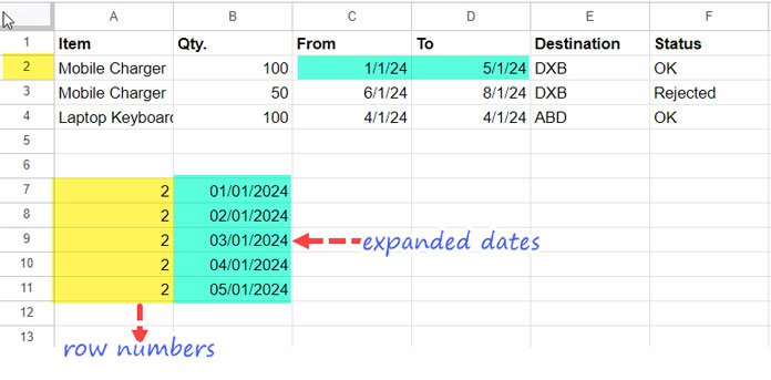
In the first part, the objective is to expand the start and end dates of the first record (row) into a single column and return the corresponding row numbers.
For example, if the start date in cell C2 is 01 Jan 2024 and the end date in cell D2 is 05 Jan 2024, expanding will yield the dates 01/Jan, 02/Jan, 03/Jan, 04/Jan, and 05 Jan.
The formula returns row numbers (e.g., 2) repeated 5 times in one column and dates 01 to 05 in another column.
These row numbers serve as search keys in VLOOKUP to retrieve values from corresponding rows in the table A2:F4. The result is horizontally appended to the expanded dates returned by the first part, creating a 7-column table.
The third part involves reordering the columns returned by the VLOOKUP, along with the dates that were appended.
The output in each iteration (each expansion) is stacked vertically using an accumulator, and that is the final result.
This logic underlies the formula that duplicates rows based on start and end dates in Google Sheets. Let’s proceed to the formula breakdown.
Formula Breakdown:
REDUCE(TOCOL(,1), C2:C4, LAMBDA(a, v, ...The REDUCE function iterates over each element in the array C2:C4 (start date column) and performs a lambda function. It takes an initial value (TOCOL(,1)) and an array (C2:C4).
Syntax:
REDUCE(initial_value, array_or_range, lambda)The initial value TOCOL(,1), essential a TOCOL function, represents an empty cell, instructing it to ignore blanks, thus preventing REDUCE from leaving an empty cell at the top of the result column.
Within the lambda, “a” is the initial value in the accumulator, and “v” is the current element in the array. The lambda function begins with VSTACK(a, indicating that REDUCE stacks the result in each iteration vertically.
Here is the explanation of the lambda function used within the REDUCE to expand dates based on the start and end dates, a key part of duplicating records.
1. SEQUENCE and IF Logical Part:
Let’s examine what the lambda function does with the first element in the array, i.e., the value in cell C2.
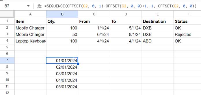
SEQUENCE(OFFSET(v, 0, 1)-OFFSET(v, 0, 0)+1, 1, OFFSET(v, 0, 0))Where:
rows:OFFSET(v, 0, 1)-OFFSET(v, 0, 0)+1equalsend_date - start_date + 1.columns: 1.start:OFFSET(v, 0, 0), representing the start date.step: omitted.
This follows the SEQUENCE syntax:
SEQUENCE(rows, [columns], [start], [step])The formula above expands the start and end dates. We use the LET function to name this value expression as “seq.”
IF(seq, ROW(v))This IF part returns row numbers corresponding to “seq.” The LET function assigns the name “lkp” to this, meaning lookup value.
2. VLOOKUP Part:
VLOOKUP(
lkp,
HSTACK(ROW(C2:C4), A2:F4),
SEQUENCE(1, COLUMNS(A2:F4), 2)
)
The VLOOKUP searches “lkp,” which is the row numbers of the expanded start and end dates, in the range HSTACK(ROW(C2:C4), A2:F4). It returns all matching records in all columns except the first column. The result is horizontally stacked with the expanded dates.
The output is named “fnl” in the LET function.
3. CHOOSECOLS Part:
CHOOSECOLS(fnl, 1, 2, 7, 5, 6)This CHOOSECOLS part selects the columns except for the start and end date columns. Instead of that, it chooses the expanded column.
This concludes the explanation of the formula designed for duplicating rows based on start and end dates in Google Sheets.
What Are the Benefits of Duplicating Rows Based on Start and End Dates in Google Sheets?
Duplicating rows based on start and end dates in Google Sheets provides several advantages. Here are the most important ones.
Focused Data Analysis:
Filtering dates allows for a focused view of data on specific days. Formulas like MONTH, YEAR, WEEKNUM, or week range in a helper column help narrow down data to specific years, months, weeks, or custom date ranges.
Related: How to Utilise Google Sheets Date Functions [Complete Guide]
Data Aggregation with Pivot Tables:
The duplicated data can be efficiently aggregated using Pivot Tables in Google Sheets. This enables aggregation by day, month, year-month, quarter, and other customizable time intervals.
Time-Saving Data Entry:
Entering data based on start and end dates saves time, and formulas can be applied to automatically expand the dataset. This simplifies the data entry process and reduces the risk of errors.
These are some immediate benefits of duplicating records by start and end dates in Google Sheets, providing enhanced data focus, analytical capabilities, and efficiency in data entry.
Conclusion
In this tutorial, we have utilized VLOOKUP with REDUCE to duplicate records based on the start and end dates. Alternatively, we can omit the use of VLOOKUP and instead depend on OFFSET for the same purpose.
However, it’s crucial to note that using OFFSET may impact the performance of the formula. We have restricted the use of OFFSET to only obtaining the start and end dates.
This limitation is necessary because REDUCE won’t handle two arrays simultaneously, preventing us from specifying both start dates and end dates in the same function.
Resources:
- How to Insert Duplicate Rows in Google Sheets
- Assign the Same Sequential Numbers to Duplicates in a List in Google Sheets
- Expand Dates and Assign Values in Google Sheets (Array Formula)


