The SUMIFS function in Google Sheets simplifies conditionally summing a range, making it a powerful tool for summarizing data.
The SUMIF function is another option for conditional summation. Use it when you need to sum based on a single criterion, whereas SUMIFS is used for multiple criteria.
As a side note, you can use SUMPRODUCT, SUM+FILTER, and QUERY to replace these two functions. However, SUMIF and SUMIFS are dedicated functions for conditional summation.
Syntax of SUMIFS in Google Sheets
SUMIFS(sum_range, criteria_range1, criterion1, [criteria_range2, criterion2, ...])- sum_range: The range that will be summed. It should contain numeric data.
- criteria_range1: The range against which the first criterion is evaluated.
- criterion1: The first criterion.
- [criteria_range2, criterion2, …]: Optional. Additional ranges and criteria to be evaluated.
Note: In SUMIF, the sum_range is the last argument. Be cautious not to mistakenly place sum_range as the last argument in SUMIFS.
SUMIFS Examples in Google Sheets
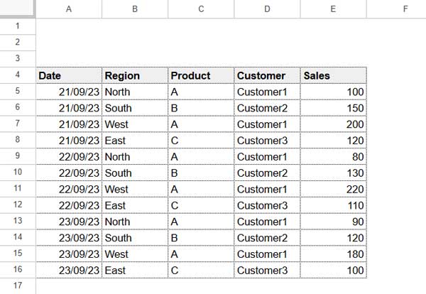
The following sample data contains sales records structured with Date, Region, Product, Customer, and Sales in columns A, B, C, D, and E, respectively. The data is stored in the range A4:E16. I have left three empty rows above for specifying the criteria.
You can make a copy of my sample sheet by clicking on the button below.
Basic SUMIFS Example
How do you sum the total sales of the product “A” in the North region?
Use the following SUMIFS formula:
=SUMIFS(E5:E, B5:B, B1, C5:C, C1)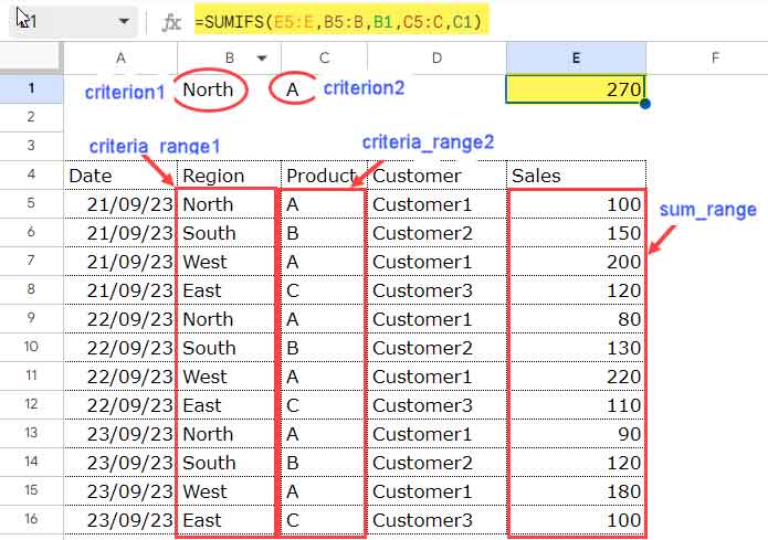
Explanation of SUMIFS Function Arguments
- E5:E: The range of values (Sales) to be summed.
- B5:B: The first criteria range (“Region” column), where values must match “North.”
- B1: The reference cell containing the value “North.”
- C5:C: The second criteria range (“Product” column), where values must match “A.”
- C1: The reference cell containing the value “A.”
To hardcode the criteria, use:
=SUMIFS(E5:E, B5:B, "North", C5:C, "A")This formula calculates the total sales amount for product “A” in the North region based on specified criteria.
Using SUMIFS with Numbers, Dates, and Text
In the above example, we used text criteria. But what about numbers, dates, and timestamps?
For a date condition in SUMIFS:
=SUMIFS(E5:E, D5:D, "Customer1", A5:A, DATE(2023, 9, 21))This formula returns the total sales amount for “Customer1” on 21/09/2023. Use the DATE function to specify date criteria correctly.
For numbers, specify them without quotes:
=SUMIFS(E5:E16, E5:E16, 100)This sums the sales where the value is exactly 100.
Fixing Common SUMIFS Limitations
SUMIFS does not support using the same criteria range multiple times unless comparison operators are used.
Example: Summing Sales Between Two Dates for Product “A”
=SUMIFS(E5:E, A5:A, ">="&DATE(2023, 9, 22), A5:A, "<="&DATE(2023, 9, 23), C5:C, "A")This works correctly.
However, this formula aiming to sum total sales for product “A” from both North and South regions will not work:
=SUMIFS(E5:E, B5:B, "North", B5:B, "South", C5:C, "A")Instead, use:
=ArrayFormula(SUMIFS(E5:E, (B5:B="North")+(B5:B="South"), 1, C5:C, "A"))Alternatively, use REGEXMATCH:
=ArrayFormula(SUMIFS(E5:E, REGEXMATCH(B5:B, "(?i)^North$|^South$"), TRUE, C5:C, "A"))Using Wildcards in SUMIFS
The SUMIFS function supports wildcards:
- Asterisk (
*): Represents zero or more characters. - Question mark (
?): Represents any single character.
=SUMIFS(E5:E, B5:B, "N*")This sums sales where the “Region” starts with “N” (e.g., “North”).
=SUMIFS(E5:E, D5:D, "Customer?")This sums values where the “Customer” column contains “Customer” followed by any one character.
To use * or ? as literal characters (not wildcards), prefix them with a tilde (~).
For example, to match the exact text *Total*:
=SUMIFS(E5:E, B5:B, "~*Total~*")This treats the asterisks as normal characters instead of wildcards.
SUMIFS with Empty or Non-Empty Cells
To sum a column based on empty cells:
=SUMIFS(E5:E, C5:C, "A", D5:D, "")For referencing an empty cell as a criterion:
=SUMIFS(E5:E, C5:C, "A", D5:D, "="&F1)For non-empty cells:
=SUMIFS(E5:E, C5:C, "A", D5:D, "<>"&F1)Practical Applications of SUMIFS
For summarizing data, consider using Pivot Tables and the QUERY function. However, SUMIFS remains a strong choice.
We often combine UNIQUE with SUMIFS. For testing, enter this formula in cell B19.
=UNIQUE(B5:D16)It will return the unique rows from the region, product, and customer columns.
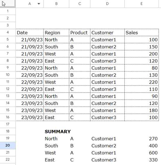
Using SUMIFS with this output:
=SUMIFS($E$5:$E$16, $B$5:$B$16, B19, $C$5:$C$16, C19, $D$5:$D$16, D19)Enter this formula in cell E19 and drag down.
Alternatively you can expand the result automatically by applying the LAMBDA as follows:
=MAP(B19:B22, C19:C22, D19:D22, LAMBDA(a, b, c, SUMIFS(E5:E16, B5:B16, a, C5:C16, b, D5:D16, c)))Troubleshooting SUMIFS Errors
If SUMIFS returns incorrect results, check the following:
- Criteria ranges must be the same size as
sum_range. sum_rangeshould not be an expression; it must be a valid range.- The function name is spelled correctly.
- Cell references are intact and not broken due to deleted columns or rows.
- Text and number formats are correct and consistent.
- Wildcards (
*,?) and logical operators (<,>,<>,=) are used properly.
Conclusion
Mastering the SUMIFS function in Google Sheets empowers you to summarize data efficiently. Key takeaways include:
- Basic and advanced SUMIFS usage.
- Handling multiple criteria and wildcards.
- Using MAP Lambda for dynamic results.
- Troubleshooting common errors.
For further reading, explore these resources:
- Using the Same Field Twice in SUMIFS in Google Sheets
- Using Different Criteria in the SUMIFS Function in Google Sheets
- REGEXMATCH in SUMIFS and Multiple Criteria Columns in Google Sheets
- How to Include a Date Range in SUMIFS in Google Sheets
- SUMIFS Array Formula for Expanding Results in Google Sheets
- SUMIF/SUMIFS Excluding Duplicate Values in Google Sheets
- SUMIFS with OR Condition in Google Sheets
- Highlight SUMIFS Rows Based on Its Total in Google Sheets
- How to Use SUMIFS to Sum Multiple Columns in Google Sheets


SO what doesn’t work is if your cell reference has a reference to another cell…ARGGGG. Even referencing the original cell on another sheet didn’t work.
In excel that wouldn’t even be a distinction that would be mentioned, because it always works, no matter how many levels of indirection there are.
I had to move my calculation to the tab where the actual text was to get this to work.
I don’t find any such issue!
See two Sumifs formulas.
Formula 1 – Criteria in another Sheet.
=sumifs(C2:C6,A2:A6,Sheet2!G2,B2:B6,Sheet2!H2)Formula 2 – Criteria in another sheet but using Indirect.
=sumifs(C2:C6,A2:A6,Sheet2!G2,B2:B6,indirect("Sheet2!H2"))Thanks.
Great example, however, what if you want to reference the same column in both arguments? Assuming “area” had East entries as well.
=sumifs(D6:D13,C6:C13,"East",C6:C13,"North")This is not working for me. I’ve tried using operators as well.
Hi Shadd,
You can use REGEXMATCH inside SUMIF to get the result that you want.
=ArrayFormula(sumif(regexmatch(C6:C13,"North|East"),TRUE,D6:D13))There are multiple options. See one more formula that using two Sumifs together.
=sumif(C6:C13,"North",D6:D13)+sumif(C6:C13,"East",D6:D13)Hope this helps.