One of the problems you may face while using functions like DSUM, SUMIFS, SUMPRODUCT, or QUERY is using the same criterion field twice.

SUMIFS and DSUM are two multiple-criteria conditional SUM functions. SUMIFS is a logical function, while DSUM is a database function.

Whether it’s SUMIFS or DSUM, you can get the same result by using the criterion in a proper way. SUMPRODUCT can also replace the other two functions in Google Sheets.

In DSUM, it’s simple to enter the criteria under field titles. However, things are more complicated when you want to include the same criteria column (criteria range) twice in SUMIFS.

There are three main approaches to using the same criteria field twice in the SUMIFS function in Google Sheets:

1. Combine two SUMIFS formulas: This approach involves adding two SUMIFS formulas together, with each formula using a different criterion in the same range.
2. Use a SUBSTITUTE workaround: This approach involves using the SUBSTITUTE function to replace one of the criteria with the other.
3. Use REGEXMATCH: This approach involves using the REGEXMATCH function to match both criteria in the same range. This will return TRUE or FALSE. We can use TRUE as the criterion.

Let’s see a few examples of this:

Syntax of the SUMIFS function in Google Sheets:

SUMIFS(sum_range, criteria_range1, criterion1, [criteria_range2, …], [criterion2, …])

SUMIFS: Same Criteria Range for Comparison

When we use date or number criteria with comparison operators in the SUMIFS function, we do not face any issues using the same criteria range twice.

For example, suppose your date range is C7:C14, you can include this date field twice in SUMIFS as criteria_range1 and criteria_range2:

=SUMIFS(D7:D14,C7:C14,">="&DATE(2017,7,1),C7:C14,"<="&DATE(2017,7,31),A7:A14,"Myron Ambriz",B7:B14,"North")

This SUMIFS formula will sum the range D7:D14 if:

• C7:C14 is greater than or equal to July 1, 2017
• C7:C14 is less than or equal to July 31, 2017
• The text in A7:A14 is “Myron Ambriz”
• The text in B7:B14 is “North”

You can enter these criteria in the cell range C1:C4 and use the formula as follows:

=SUMIFS(D7:D14,C7:C14,">="&C1,C7:C14,"<="&C2,A7:A14,C3,B7:B14,C4)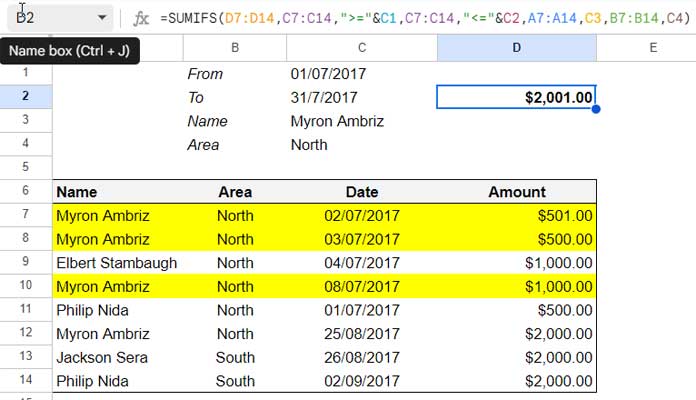

Let me explain how to deal with the same criteria range twice when there are no comparison operators.

Different Methods to Include the Same Field Twice in the SUMIFS Function

This is the interesting part. In this section, you can learn the different methods we mentioned at the beginning for including the same field (criteria range) twice in SUMIFS in Google Sheets.

Problem: How to use SUMIFS to sum the sales amount (C7:C14) of “Philip Nida” (A7:A14) in “North” or “South” (B7:B14)?

Method 1: Combine Two SUMIFS Formulas

Let’s start with the simplest form to use the same criteria field twice, which is combining two SUMIFS formulas.

This approach involves adding two SUMIFS formulas together:

=SUMIFS(C7:C,A7:A,"Philip Nida",B7:B,"North")+
SUMIFS(C7:C,A7:A,"Philip Nida",B7:B,"South")

This formula replaces the hardcoded criterion with cell references:

=SUMIFS(C7:C,A7:A,C1,B7:B,C2)+
SUMIFS(C7:C,A7:A,C1,B7:B,C3)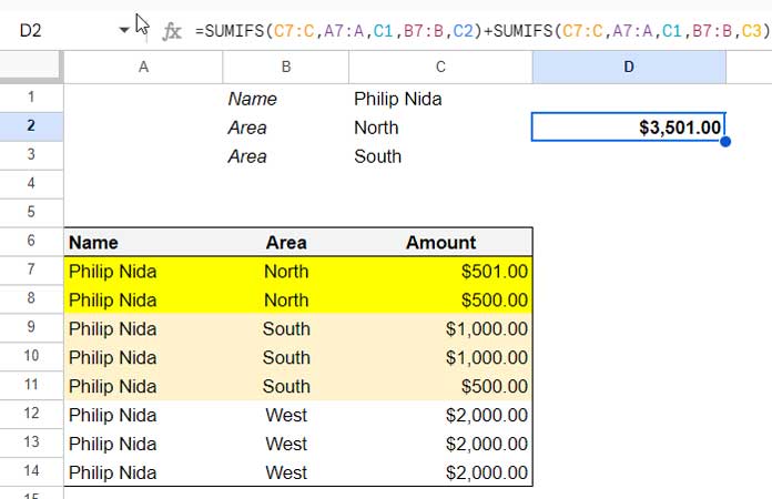

Method 2: Use a SUBSTITUTE Workaround

This approach involves using the SUBSTITUTE function to replace one of the criteria with the other.

For example, to sum the values in C7:C14 where the values in A7:A14 is “Philip Nida” and B7:B14 is “North” or “South”, you could use the following formula:

=ArrayFormula(SUMIFS(C7:C14,A7:A14,"Philip Nida",SUBSTITUTE(B7:B14,"South","North"),"North"))

We have used the SUBSTITUTE function to replace “South” with “North” in column B. So essentially, we do not need to use the same criteria field twice in the SUMIFS function.

The SUBSTITUTE function requires ARRAYFORMULA support.

The same SUMIFS formula with hardcoded criteria replaced with cell references:

=ArrayFormula(SUMIFS(C7:C,A7:A,C1,SUBSTITUTE(B7:B,C3,C2),C2))

Method 3: Use REGEXMATCH

This approach involves using the REGEXMATCH function to match both criteria in the same range. This will return TRUE for matching rows, which will be used as the criterion.

For example, to sum the values in C where the values in column A is “Philip Nida” and B is “North” or “South”, you could use the following formula:

=ArrayFormula(SUMIFS(C7:C14,A7:A14,"Philip Nida",REGEXMATCH(B7:B14, "North|South"),TRUE))

The same formula with the criterion replaced with cell references:

=ArrayFormula(SUMIFS(C7:C14,A7:A14,C1,REGEXMATCH(B7:B14, C2&"|"&C3),TRUE))

Related: REGEXMATCH in SUMIFS and Multiple Criteria Columns in Google Sheets.

Which Method is the Most Effective for Using the Same Field Twice in the SUMIFS Function?

Of the three methods, I prefer REGEXMATCH (method #3). When you want to use the same criteria field more than once, it is easy to include the criteria by simply separating them with a pipe.

The SUBSTITUTE method #2 requires multiple nesting depending on the number of criteria.

The SUMIFS method #1 may require adding more than one SUMIFS formula, which can make the formula cluttered.

In conclusion, the SUMIFS formula does not support using the same criteria field more than once without comparison operators.

In the SUBSTITUTE method, we replace one criterion with the other, so there is essentially only one criterion. When using REGEXMATCH, we use the criterion TRUE, which is also only one criterion.