If you heavily rely on SUMIFS to conditionally sum columns, you should learn how to use REGEXMATCH in SUMIFS.
SUMIFS is not required to perform multiple conditional sums. Other functions, such as QUERY and SUMPRODUCT, can also do the job. However, I know that some of you are not familiar with these two functions.
When it comes to multiple criteria in the same column, you can use SUMIF. It is the simplest solution available.
But what about multiple conditions in the same column plus additional conditions from other columns together?
Let me walk you through some examples.
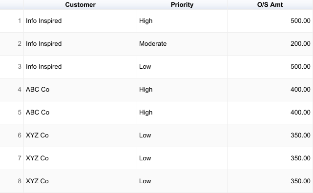
In the following example, I have customer names in column A, payment priorities (High, Moderate, and Low) in column B, and outstanding amounts in column C.
Let’s conditionally sum the outstanding amounts.
Multiple Conditions in the Same Column in Conditional Sum in Google Sheets
To sum based on multiple conditions in the same column in Google Sheets, you can use the SUMIF function with the ARRAYFORMULA function.
For example, the following formula will sum the values in column C where the Priority in column B is either “High” or “Moderate”:
=ARRAYFORMULA(
   SUM(
      SUMIF(B2:B,{"High";"Moderate"},C2:C)
   )
)
Note: You can replace {"High";"Moderate"} with VSTACK("High","Moderate") or HSTACK("High","Moderate").
The SUMIF function sums the values in a range based on a single criterion.
The ARRAYFORMULA function allows you to apply the SUMIF function to an array of values, which is necessary when you are summing multiple criteria in the same column.
The output will be in multiple cells, which the SUM function will aggregate.
Multiple Criteria in the Same Column and Another Column in Conditional SUM
In this example, you want to sum the O/S Amt (column C) for the Customer (column A) “Info Inspired” if the Priority (column B) is “High” or “Moderate.”
SUMIF is not a good solution here because it would become complex.
SUMIFS supports multiple criteria in conditional sums, but it does not support the curly bracket or VSTACK/HSTACK approach similar to SUMIF.
This means that you cannot include multiple criteria inside curly brackets or VSTACK/HSTACK in SUMIFS.
One solution is to use multiple SUMIFS formulas, but this is not recommended. A better solution is to use REGEXMATCH in SUMIFS.
How to Use REGEXMATCH in SUMIFS to Handle Multiple Criteria Columns
To use REGEXMATCH in SUMIFS to handle multiple criteria columns, you can use the following steps:
- Create a regular expression that matches the conditions for the column that you want to filter. To do this, simply list your criteria separated by pipes (
|). For example, the regular expression"High|Moderate"will match any value in the column that is equal to “High” or “Moderate”. - Use the REGEXMATCH function to test the values in the column against the regular expression. The syntax for the REGEXMATCH function is
REGEXMATCH(text, regular_expression). For example, the following formula will return TRUE if the value in cell B2 matches the regular expression “High|Moderate”:
=REGEXMATCH(B2, "High|Moderate")- Use the SUMIFS function to sum the values in the column that you want to sum, based on the results (Boolean TRUE / FALSE) of the REGEXMATCH function. The syntax for the SUMIFS function is
SUMIFS(sum_range, criteria_range1, criterion1, [criteria_range2, criterion2], …).
For example, the following formula will sum the values in column C for the Customer “Info Inspired” if the Priority in column B is “High” or “Moderate”:
=ARRAYFORMULA(
    SUMIFS(
       C2:C9,
       A2:A9, "Info Inspired",
       REGEXMATCH(B2:B9,"High|Moderate"), TRUE
   )
)
REGEXMATCH in SUMIFS: Formula Explanation
In the above formula, the arguments used are as follows.
Sum_range:C2:C9Criteria_range1:A2:A9Criterion1:"Info Inspired"Criteria_range2:REGEXMATCH(B2:B9, "High|Moderate")Criterion2:TRUE
Explanation:
We need to use two conditions in column B. The SUMIFS function does not support multiple criteria in the same column. So we can’t use B2:B9 twice.
To address this limitation, we can use the REGEXMATCH function. It will match both the criterion in column B and return an array with TRUE/FALSE values.
So the criteria range will be the REGEXMATCH returned Boolean values and the criterion will be TRUE.
Here is another formula where we use three conditions in the same column using REGEXMATCH in SUMIFS.
=ARRAYFORMULA(
    SUMIFS(
       C2:C9,
       A2:A9, "Info Inspired",
       REGEXMATCH(B2:B9,"High|Moderate|Low"), TRUE
   )
)
That’s all!
This way, you can use REGEXMATCH in SUMIFS in Google Sheets to sum values based on multiple criteria in the same column.
Share this tip!


Sure, where can we communicate?
Hi, Reu Hadrian Ceballos,
You can share your ‘editable’ SHEETS’ URL below using the comment form. I won’t publish it.
“The result was not automatically expanded, please insert more rows (39438).”
=arrayformula(sumif(TransID!D2:D40000,regexmatch(TransID!B2:B40000,"642812004978|19834993968|4102897003990|29170106066")))
Hi, Reu Hadrian Ceballos,
The Syntax seems incorrect. Sumif evaluates the criteria in the “range”. In your case, both are different arrays/ranges.
If you want me to try to troubleshoot, you may require to share an example sheet.
Can we use a cell reference in Regexmatch? If so, what should be the formula to use?
Hi, An,
If cell range D2:D4 contains the criteria High, Moderate and Low, we can replace the last formula in my tutorial with the below one.
=ArrayFormula(sumifs(C2:C9,A2:A9,"Info Inspired",REGEXMATCH(B2:B9,textjoin("|",true,D2:D4)),TRUE))Hi Prashanth,
Happy new year to you.
I am trying to use a formula to sum values where the column next to it contains a text string. The following works to do this:
=ArrayFormula(sum(sumif(regexmatch(lower('DATA ARRAY'!C:C),Lower(A4)),TRUE,'DATA ARRAY'!D:D)))However, I have to copy this formula down every time a new row is added, but I want to document to be automated. I thought I could have this formula copy down automatically by using the following:
=arrayformula(IF(NOT(ISBLANK($A4:A)), sum(sumif(regexmatch(lower('DATA ARRAY'!C:C),Lower(A4:A)),TRUE,'DATA ARRAY'!D:D)),))This [IF NOT ISBLANK] addition works when I want a VLOOKUP function to work automatically as data is added in the next row of the document. However, in this case, it causes every line to sum all the numbers in the sum range, instead of only looking up the value in the cell next to it. Do you know if it is fixable?
Best,
Holly
Hi, Holly,
Issues in your formula.
1. The SUM function makes the formula non-array.
2. You can simplify the SUMIF formula using wildcards instead of using the REGEXMATCH text function.
So you can try this SUMIF array formula.
=ArrayFormula(if(len(A4:A),(sumif('DATA ARRAY'!C:C,"*"&A4:A&"*",'DATA ARRAY'!D:D)),))Hi,
I’m trying to exclude percentage values in my Sumifs formula (among other things). But I’ve been wracking my brain trying to figure out how to do so without it simply defaulting to a decimal value.
Do you have any suggestions as to what I could do?
Thank you for your time.
You may need to use a helper array/range as the sum_range in SUMIFS can’t be an expression.
You can use something like this in the helper range (insert in D2 after making D2:D10 blank) to extract numbers from C2:C10.
=ArrayFormula(if(iferror(search("%",C2:C10))="",C2:C10,))or this more refined Regex one.
=ArrayFormula(IFNA(if(iferror(search("%",C2:C10))="",REGEXEXTRACT(to_text(C2:C10), "([0-9]+)")*1,)))Hi,
Getting “Formula parse error en 2019” with the last formula.
Hi, Tomas,
It may be due to regional settings. Try this instead.
=ArrayFormula(sumifs(C2:C9;A2:A9;"Info Inspired";regexmatch(B2:B9;"High|Moderate|Low");TRUE))