If you are looking for a flexible array formula to join columns in Google Sheets, you are in the right spot! I’ve two best solutions.

We can join columns with a basic Query formula that only uses the header argument. Yep! You have heard me correctly.

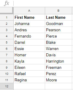
For example, we usually depend on the available text functions to combine first and last names in two columns.

What are they?

They are Join, Text Join, Concat, and Concatenate. But none of them supports arrays the way we want. We will see examples of this later on.

Update:- We can now use these text functions with a supporting Lambda to work as required. I’ll add those solutions at the end of this tutorial.

The only option left with us is the ampersand sign which requires physical columns. If we have a five columns array returned by a Filter formula, to join, we must first take out each column.

But I have a simple and elegant solution using a Query that will work with physical, as well as, virtual columns.

I want to join these names in a third column.

Let’s check some of the formulas we usually use to combine text. Then we can go to the ultimate solution.

Similar: Stack Data in Google Sheets – Spreadsheet Tips and Tricks

Join Columns Using Join, Textjoin, and Concatenate Functions

Insert any of the following formulas in cell C2 and copy-paste it down.

We will start with the Join function.

=JOIN(" ",A2:B2)

The following Concatenate works similarly.

=CONCATENATE(A2," ",B2)

In the above two formulas, space is the delimiter that separates the first and last names.

What about this Textjoin?

=textjoin(" ",TRUE,A2:B2)

It’s also a drag-down (copy-paste) formula and space character used as the delimiter.

But, it has an added advantage.

The formula won’t add the delimiter if you forget to enter the first or last name. So the output will look nice.

All the above are non-array formulas to join columns in Google Sheets. We can convert them to array formulas using a Lambda function, though. We will see that later.

Two Array Formulas Using Concat and Ampersand

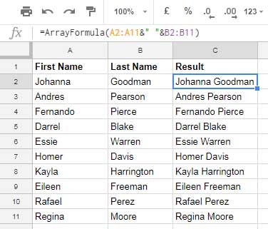
I may recommend ampersand use if you ask me which is the easiest array formula method to join columns in Google Sheets.

=ArrayFormula(A2:A11&" "&B2:B11)

This Concat will also work but only with two columns. So, it’s not an ideal way!

=ArrayFormula(concat(A2:A11&" ",B2:B11))

The first formula using ampersand has its drawback too. What are they?

If you insert a new column between columns A and B and want to join the three columns, you should manually modify the formula.

For example, I’ve inserted a new column that contains the middle name.
But the formula would only join the first name and last name.

Another issue is we can’t use expressions (virtual columns). Do you want an example of this? Here you go!

With a Filter and Regexmatch combo, we can filter all the names in column A, starting with the letter “E.”

=filter(A2:B11,regexmatch(A2:A11,"(?i)E"))

The formula will return the following names.

What about filtering and combining altogether?

Let’s do that using my flexible array formula that joins columns.

1. Flexible Array Formula to Join Columns in Google Sheets – QUERY

First, let us see the formula.

=transpose(query(transpose(A2:B11),,COLUMNS(A2:B11)))

If you want to use an expression, for example, a filter as mentioned earlier, instead of A2:B11, use the filter formula.

=transpose(query(transpose(filter(A2:B11,regexmatch(A2:A11,"(?i)E"))),,COLUMNS(A2:B11)))

Anatomy of the Formula

See the syntax: QUERY(data, query, [headers])

If you use any data in the Query formula without a query, it will return the data as it is.

In our Query, transposed range B2:B11 is the data.

=query(transpose(A2:B11))

We have transposed two columns. So we have two rows.

We will tell the Query that these two rows are headers.

=query(transpose(A2:B11),,2)

We will get the following result.

Instead of hardcoding # 2, we can use the Columns function to dynamically return the number of columns in the data range A2:B11 (number of rows in the transposed data range A2:B11).

That’s what I did. Then transposed the data once again.

2. Flexible Array Formula to Join Columns in Google Sheets – BYROW

Using Byrow, one of the Lambda helper functions, we can expand the result of the text functions mentioned at the beginning of this tutorial.

Here I am selecting Textjoin, as it can omit blank cells.

Here is the second flexible array formula to join columns in Google Sheets.

=byrow(A2:B11,lambda(r,textjoin(" ",true,r)))

That’s all. Thanks for the stay. Enjoy!