You can use the VSTACK function to vertically combine two or more tables with unequal columns in the QUERY function in Google Sheets.
VSTACK is a relatively new function. Previously, we used a method to make the column sizes virtually equal so that QUERY would work correctly.
Combining two or more tables in the QUERY data is an important task when you want to aggregate data from multiple sheets in the same file. VSTACK makes this much easier.
Combining Tables in QUERY and Handling Mixed Data Types
Before we go into the steps to combine tables in QUERY, you must understand one important thing:
If column A is a text column, B is a date column, and C is a numeric column in one table, the same data types must be in the corresponding columns of the second table.
Otherwise, the QUERY function will return incorrect results. More precisely, QUERY takes the majority data type of the concerned column for query purposes, and minority data types are considered null values.
Example of Combining Tables with Unequal Columns in QUERY
In this example, Table 1 in Sheet1 contains the following data for one salesperson:
| Product | January | February |
| Product 1 | 15 | 20 |
| Product 2 | 20 | 25 |
| Product 3 | 25 | 20 |
The data range is A1:C4, where A1:C1 contains the field labels Product, January, and February.
Table 2 in Sheet2 contains the following data in A1:D5, with field labels Product, January, February, and March in A1:D1. This represents the sales data of another person.
| Product | January | February | March |
| Product 1 | 25 | 40 | |
| Product 2 | 30 | 40 | |
| Product 3 | 30 | 35 | 35 |
| Product 4 | 35 | 40 | 0 |
The number of columns in these two tables is different. Here’s how to properly combine them and prepare for aggregation.
Step 1: Stacking Vertically
When stacking, start with the actual range first, like A2:C4 (Table 1) and A2:D5 (Sheet2). Later, you can expand them to A2:C and A2:D to accommodate future data entries in these tables.
Also, exclude the header row initially. Headers can be added later.
=VSTACK(Sheet1!A2:C4, Sheet2!A2:D5)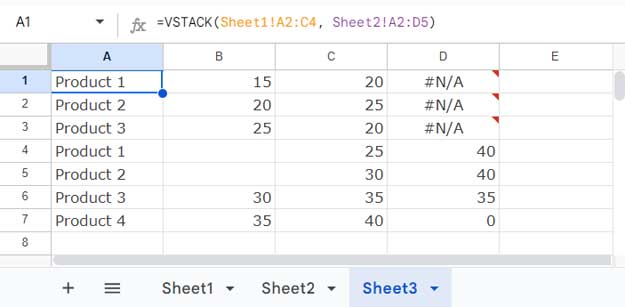
This VSTACK formula combines the two tables for use in QUERY. If a table has fewer columns than the maximum width of the selected tables, Sheets returns a #N/A error in the additional columns.
Step 2: Removing #N/A Errors
To remove #N/A errors, wrap the VSTACK formula with the IFNA function:
=IFNA(VSTACK(Sheet1!A2:C4, Sheet2!A2:D5))Step 3: Adding the Field Labels
Manually specify the field labels and stack them at the top of the combined table. First, determine the number of columns in your larger table (Table 2 has 4 columns).
Here’s an example array with 4 field labels:
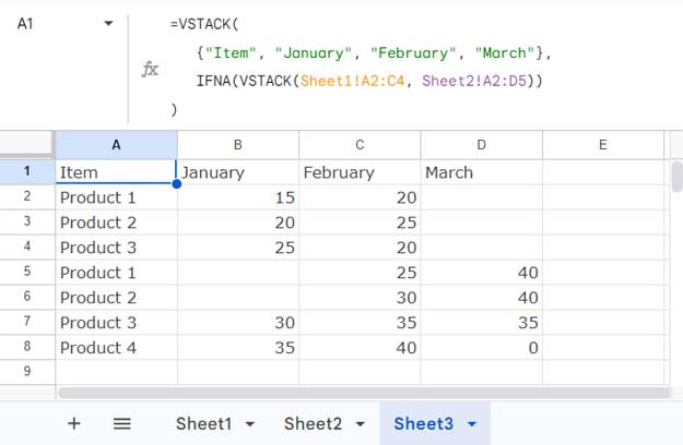
{"Item", "January", "February", "March"}Combine them with the combined table using VSTACK:
=VSTACK(
   {"Item", "January", "February", "March"},
   IFNA(VSTACK(Sheet1!A2:C4, Sheet2!A2:D5))
)
Step 4: Combining Two Tables with Unequal Columns in QUERY
Here’s the final step where we use the combined table within the QUERY function, expanding the ranges:
Syntax:
QUERY(data, query, [headers])Now let’s use the combined table:
Example 1: Select all columns in the combined table
=QUERY(
   VSTACK(
      {"Item", "January", "February", "March"},
      IFNA(VSTACK(Sheet1!A2:C4, Sheet2!A2:D5))
   ),
   "SELECT *", 1
)
Example 2: Select all columns and filter out blank rows based on the first column
Now it’s time to adjust the ranges A2:C4 and A2:D5.
=QUERY(
   VSTACK(
      {"Item", "January", "February", "March"},
      IFNA(VSTACK(Sheet1!A2:C, Sheet2!A2:D))
   ),
   "SELECT * WHERE Col1 IS NOT NULL", 1
)
Opening the range too broadly beforehand could result in each table being populated with hundreds of blank rows, potentially leading to issues.
This method allows combining tables with unequal columns in the data part of the QUERY function effectively.
Combining and Consolidating Two Tables with Different Numbers of Columns
In the combined table, you can manipulate the query string for tasks like sorting, aggregating, pivoting, and more.
Replace
"SELECT * WHERE Col1 IS NOT NULL"with
"SELECT * WHERE Col1 IS NOT NULL ORDER BY Col1 ASC"to sort the combined tables by the first column in ascending order.
Do you want to group the first column and aggregate the data?
Then use this query string:
"SELECT Col1, SUM(Col2), SUM(Col3), SUM(Col4) WHERE Col1 IS NOT NULL GROUP BY Col1 ORDER BY Col1 ASC"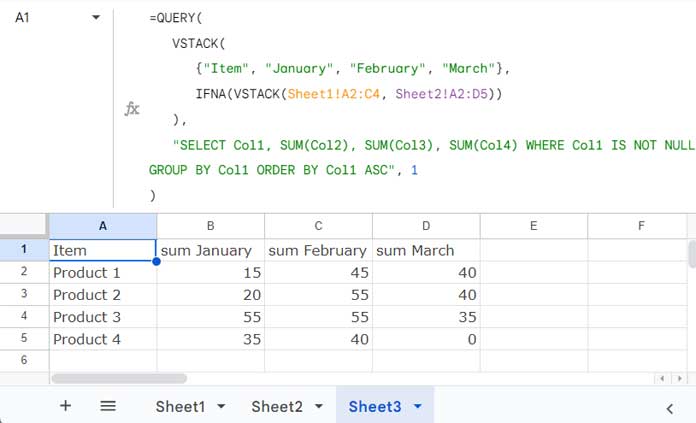
You have learned a powerful technique for combining two tables with unequal columns using QUERY and creating a master table where you can access summarized data from other sheets.
Resources
- How to Combine Two Query Results in Google Sheets
- Query to Combine Columns and Adding Separators in Google Sheets
- How to Left Join Two Tables in Google Sheets
- How to Right Join Two Tables in Google Sheets
- How to Inner Join Two Tables in Google Sheets
- How to Full Join Two Tables in Google Sheets
- Master Joins in Google Sheets (Left, Right, Inner, & Full) – Duplicate IDs Solved
- Anti-Join in Google Sheets: Find Unmatched Records Easily


Could you explain formula #1 in more detail? Specifically,
IFERROR({Sheet1!A3:C, " "/ROW(Sheet1!A3:A)}, 0)? There is no explanation, and it looks odd.Using
" "/ROW(Sheet1!A3:A)formula part with ARRAYFORMULA like=ARRAYFORMULA(" "/ROW(Sheet1!A3:A))returns error values. IFERROR converts those errors to 0, effectively adding an extra column containing 0’s.However, this approach is no longer necessary. I’ve updated the tutorial to include a much simpler solution.