I get cool ideas from my occasional interaction with my blog users. How to insert blank columns in Google Sheets QUERY is one of them.
We can easily insert single or multiple blank columns in a Google Sheets QUERY formula result. However, if you don’t follow certain steps, it can get a bit tricky.
Specifically, the formula will vary depending on whether you have headers in your QUERY result. Additionally, the method of adding columns will differ based on the number of columns.
Let’s delve into these concepts with examples using the sample data provided below.
The sample data consists of four columns: Date, Item, Category, and Region, arranged in cell range A1:D. The field labels are in the cell range A1:D1.
| Date | Item | Category | Region |
| 15/3/24 | Item 1 | Category 1 | North |
| 15/3/24 | Item 1 | Category 2 | North |
| 15/3/24 | Item 2 | Category 3 | North |
| 15/3/24 | Item 1 | Category 4 | North |
| 20/3/24 | Item 2 | Category 1 | South |
| 20/3/24 | Item 1 | Category 2 | South |
| 20/3/24 | Item 1 | Category 3 | South |
| 20/3/24 | Item 2 | Category 4 | South |
| 25/3/24 | Item 2 | Category 1 | East |
| 25/3/24 | Item 2 | Category 2 | East |
| 25/3/24 | Item 1 | Category 3 | East |
The following QUERY formula filters for “Category 1”:
=QUERY({A1:D}, "SELECT Col1, Col2, Col3, Col4 WHERE Col3='Category 1' ", 1)How can we incorporate blank columns into the result of this QUERY formula?
Inserting Blank Columns to a QUERY Result with a Header Row
To insert blank columns, use space characters in the SELECT clause within the QUERY function.
For the first column, use one space; for the second column, use two consecutive spaces; for the third column, use three consecutive spaces, and so forth.
Additionally, it’s essential to specify the headers using the LABEL clause.
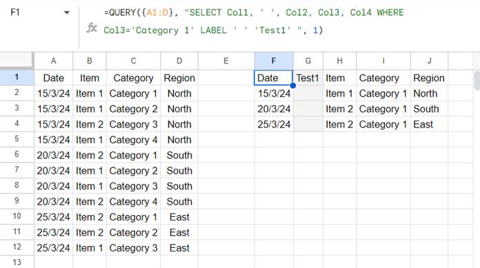
The following formula inserts a blank column after column 1 (Date), labeled “Test 1”:
=QUERY({A1:D}, "SELECT Col1, ' ', Col2, Col3, Col4 WHERE Col3='Category 1' LABEL ' ' 'Test1' ", 1)Please refer to the yellow and cyan highlighting to observe the changes made when inserting blank columns in the formula.
To insert a second blank column after the “Item” column, use this formula:
=QUERY({A1:D}, "SELECT Col1, ' ', Col2, ' ', Col3, Col4 WHERE Col3='Category 1' LABEL ' ' 'Test1', ' ' 'Test2' ", 1)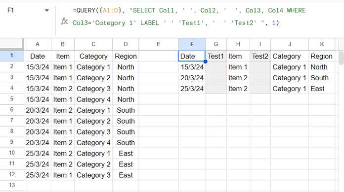
When you want to add a third blank column, use three consecutive space characters. I hope you understand the logic behind this.
Please note that the LABEL clause is the second to last clause in the Google Sheets QUERY function. The only clause that comes after this is the FORMAT clause.
Related: What is the Correct Clause Order in Google Sheets Query?
Inserting Blank Columns to a QUERY Result without a Header Row
As far as I know, the QUERY function is the only function in Google Sheets that can recognize field labels (header rows). Its syntax includes an optional third argument called ‘headers’:
Syntax: QUERY(data, query, [headers])
In the examples provided, since we have a header row, we specify 1 in headers. If there’s no header row, you can specify 0. If you omit the headers argument, the function will often try interpreting it based on the data.
In a scenario where the output doesn’t have a header row, as demonstrated in the following formula filtering for “Category 1”:
=QUERY({A2:D}, "SELECT Col1, Col2, Col3, Col4 WHERE Col3='Category 1' ", 0)When inserting blank columns in this case, you should specify '' as the label in the LABEL clause:
For inserting one blank column:
=QUERY({A2:D}, "SELECT Col1, ' ', Col2, Col3, Col4 WHERE Col3='Category 1' LABEL ' ' '' ", 0)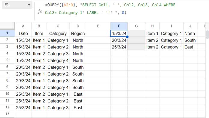
For inserting two blank columns:
=QUERY({A2:D}, "SELECT Col1, ' ', Col2, ' ', Col3, Col4 WHERE Col3='Category 1' LABEL ' ' '', ' ' '' ", 0)If you do not use the LABEL clause, the formula will leave the labels " "(), " "(), … depending on the number of columns.
Key Reminders
You have learned to add blank columns to QUERY formula results. However, if you enter any value in that blank column, the formula may break!
Then what is the purpose of adding blank columns?
It serves two purposes:
- Enhance the readability of your results by minimizing clutter.
- When printing, the hardcopy provides spaces to fill values such as leaving user comments, checkmarks, etc.
If you are particular about adding values in the QUERY results within Sheets, copy the result and paste it as values. The “paste value” option is available within the context menu, which you can access by right-clicking.
Resources
- Replace Blank Cells with 0 in Query Pivot in Google Sheets
- Filter Out Blank Columns in Google Sheets Using Query Formula
- How to Insert Blank Rows Using a Formula in Google Sheets
- How to Automatically Insert a Blank Row below Each Group in Google Sheets
- Insert Subtotal Rows in a Google Sheets Query Table
- Insert Blank Rows to Separate Week Starts/Ends in Google Sheets


Hi,
@ Prashanth: Thank you for sharing your knowledge.
I did not get, how
{" "," "}/row(A2:A)adds 2 columns specifically the/row(A2:A)part with the/symbol.Thanks
Hi, Dinesh,
To understand that, please follow the below steps.
In two blank cells, for example, in cells A1 and B1, tap the space bar to get a space character in that cells.
Now in cell C1 key in
=ArrayFormula(A1:B1/row(A1:B1)).You will get two error values in C1 and D1. Just wrap that formula with IFERROR as below.
=
ArrayFormula(IFERROR(A1:B1/row(A1:B1)))Hi, could it possible for you to put the sample data into the tutorial as text so that we can quickly copy and paste it into Sheets to try for ourselves?
Hi, Helmanfrow,
Thanks for your suggestion.
In my latest tutorials, I am trying to include example sheets wherever necessary. I’ll try to update my earlier tutorials.
The problem is, there are 1000+ posts, and it will be a time taking exercise for me to go through them all.
Hello,
Can we edit the blank column and place any number against the result of the query function, so that every time data gets change, that specific number comes against the resulted query.
Hi, Zeeshan Ali,
It’s not possible. If you want to enter any value in the blank column, first you must copy (Ctrl+C) and paste value (Ctrl+Shift+V) the result.