This tutorial explains how to use the Label clause in the Google Sheets Query function. Let’s start with its purpose.
The purpose of the Label clause in Google Sheets Query is to set or remove existing labels for one or more columns in a Query formula output.
You can set labels for the following items.
- Any columns in the data range.
- The output of aggregation functions, scalar functions, or arithmetic operators.
As a side note, other than the Label keyword, there are a few other clauses in Query.
You must adhere to the clause order if there is more than one clause in a single Query formula.
Basic: Label Columns Using the Label Clause in the Query Function
This “basic use” section will help you understand how to use the Query Label clause in Google Sheets.
In real life, you may find this handy to rename output columns of Query aggregation and scalar functions or arithmetic operators.
I’ll detail that under the advanced section after a few paragraphs below.
1. Label Clause to Set One Label in Google Sheets Query
Syntax:
label column_id label_stringcolumn_id: The column identifier (example A or Col1).
If your Query data (range) is a physical range like A1:Z, the column identifier (column_id) will be capital letters like A, B, C, etc.
But when you use an expression as the data, it will become Col1, Col2, Col3, etc.
You will get examples of this use in the advanced section below.
label_string: The label to assign to the specified column_id.
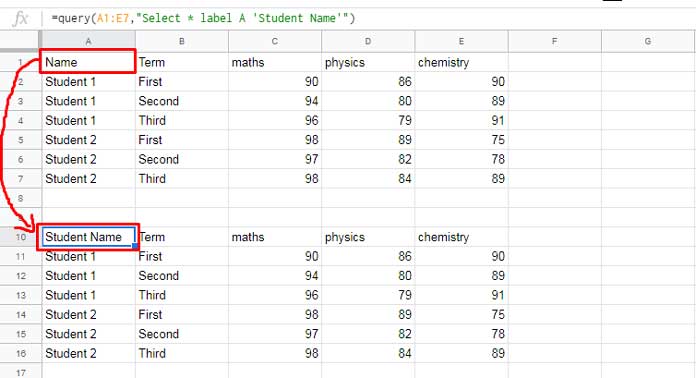
Here is an example of how to set a Label for a single column in Query.
Again, this example is just to make you understand how to use the Label clause in Google Sheets Query. In real life, you may not want to use this.
Example:
2. Label Clause to Set Multiple Labels in Google Sheets Query
Syntax:
label column_id label_string [,column_id label_string]I’ve already explained the arguments above. Here, let’s take care of how to use the optional arguments (additional column labeling).
When you change the label of multiple columns, you should use the keyword only once. Please see the following example.
There are five columns in my sample data with field labels “Name”, “Term”, “maths”, “physics”, and “chemistry”.
The following Query formula uses the one Label keyword to customize/replace/modify the labels of the last three columns (columns C, D, and E).
=query(A1:E7,"Select * label C 'Subject 1', D 'Subject 2', E 'Subject 3'")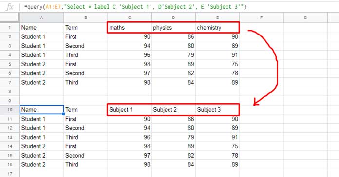
The formula retains the first two field labels, i.e., “Name” and “Term,” as it is.
What does that mean?
- You can set labels for any, all, or specified columns in the Query result.
- The columns (column identifier) left used in the Label clause part will retain their original labels.
Advanced: Label Clause in Query Aggregation, Scalar Functions, and Operators
1. Remove or Modify Headers of Aggregation Function Output in Query
I hope you are familiar with the aggregation functions in Query. If not, please refer to this guide – How to Sum, Avg, Count, Max, and Min in Google Sheets Query.
Here are the two key points that you should remember to modify labels of columns specified within the aggregation functions in Query.
- Aggregation functions take a single-column identifier as an argument. For example,
sum(B)orsum(Col2). - When using aggregation functions in the Select clause, the header of the result column should be in the format
function_name label.
Example:
=query(A1:B14,"Select sum(B)")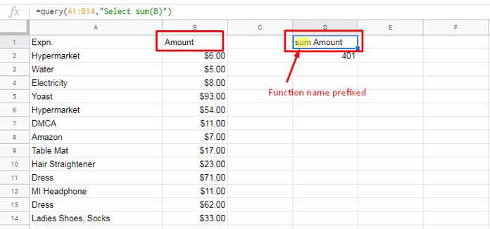
Please follow the below formula to know how to customize this header in cell D1 using the Label clause in Google Sheets Query.
=query(A1:B14,"Select sum(B) label sum(B) 'Total Amount'")What if I have an expression instead of the physical data range A1:B14?
Here, I have two examples to show you the use of ‘expressions’ as the ‘data’ in the Query function in Google Sheets.
Example of Expression as Query Data
Let me combine two data ranges to use as ‘data’ and then total the second column using Query.
=Query({A1:B10;D1:E5},"Select Sum(Col2) label Sum(Col2) 'Total Amount'")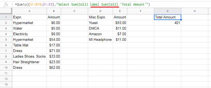
Note:- We can replace now the expression {A1:B10;D1:E5} with vstack(A1:B10,D1:E5). Find more about the VSTACK function here.
Use the above tips when using the Label clause with Query aggregation functions.
Let’s go to the second example.
How to Remove the Query Headers/Labels When Aggregation Function in Use?
To remove Query headers when using aggregation functions, use the Label clause in Query as below.
The below formula is based on the just above example. It will return the total in a single cell without a label/header.
=Query({A1:B10;D1:E5},"Select Sum(Col2) label Sum(Col2) '' ")Label Clause in Query Importrange:
=query(importrange("URL Here","Sheet1!A1:J10"),"select sum(Col10) where Col5='Student 1' label sum(Col10)''")Without the Label clause, the output of the above formula will be in two rows (two cells): One cell with the label and the second cell with the sum amount. The Label clause restricts the output to a single cell.
2. Remove or Modify Headers of Scalar Function Output in Query
The following are the scalar functions in Google Sheets Query.
- year(), month(), day(), dayOfWeek(), quarter(), dateDiff(), toDate()
- now(), hour(), minute(), second(), millisecond()
- upper(), lower()
Though I don’t have a single post featuring all of these functions, you can find most of them by searching on this site. I may consider writing a tutorial/reference guide on these functions soon.
When we come back to our topic, which is the use of the Label clause in Google Sheets Query, here is one example of the use of Label with the scalar function year().
It’s rare to see the use of the Label clause with scalar functions (alone).
It usually appears in combination with aggregation functions, and here is one example.
Example:
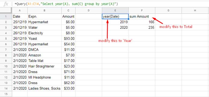
In this result, you may want to modify two labels: ‘year(Date)’ and ‘sum Amount.’ Here is how to do it.
=Query(A1:C14,"Select year(A), sum(C) group by year(A) label year(A) 'Year',Sum(C)'Total'")Tip: First, use Query formulas without the Label clause. Then take a look at the Query header. You can then easily understand how to correctly use the Label clause in Query to modify/remove the headers.
How to Remove the Query Headers/Labels When Scalar Function in Use?
All you want to do is use blank label(s) by specifying two single quotes as below.
=Query(A1:C14,"Select year(A), sum(C) group by year(A) label year(A) '',Sum(C)'' ")It removes the two labels, and that causes the result to move one row up.
3. Remove or Modify Headers of Operator Formula Output in Query
I find using the Query Label clause a must when using the arithmetic operators (see the list below) as it (operators) makes the Query headers nearly tough to read.
- Addition
(+) - Subtraction
(-) - Multiplication
(*) - and Division
(/).
Here is an example Query formula without the said clause, and after seeing it, I hope you will agree with me.
=Query(A1:E7,"Select A, C+D+E")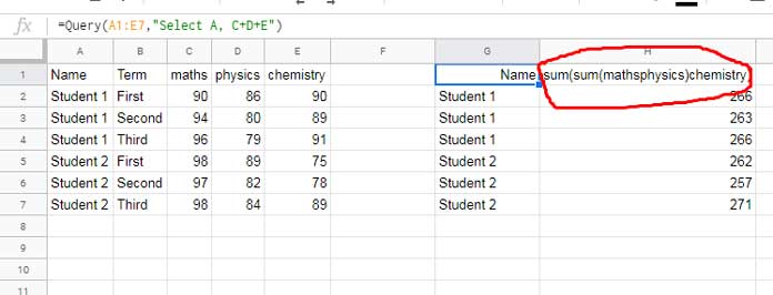
To replace the header sum(sum(mathsphysics)chemistry) with Total, use the below formula.
=Query(A1:E7,"Select A, C+D+E label C+D+E 'Total' ")How to Remove the Query Headers/Labels When Operators in Use?
I hope the below formula is self-explanatory.
=Query(A1:E7,"Select A, C+D+E label C+D+E'' ")Can I Use Label Clause to Modify the Query Pivot Header?
Yes! To modify a Query formula Pivot Header do as follows.
Wrap the Query formula that Pivots with another Query formula. In the second Query, use the Label clause.
You May Like:- How to Use Nested Queries in Google Sheets.
Didn’t get it? Then follow this example.
Query Pivot:
=query(A1:F7,"Select A, sum(F) group by A Pivot B")Query Pivot with Query Label Clause:
=query(query(A1:F7,"Select A, sum(F) group by A Pivot B"),"Select * label Col2'Term I',Col3'Term II',Col4'Term III'")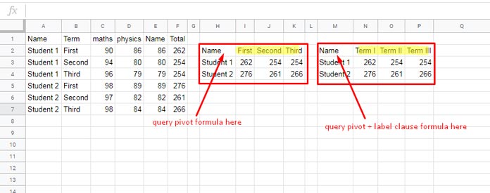
This, way you can modify the labels/headers in Query Pivot.
Related: How to Format Query Pivot Header Row in Google Sheets.


Good morning,
Thanks for these great examples.
I can’t replace the months in figures in my formula with their names.
Thanks for the help.
Hi, Terrasson,
You can’t format
month(A)+1to month names.I suggest converting column A dates to month-end dates using the EOMONTH function.
Then you can use A instead of the
month(A)+1to group or aggregate. Then you can format it into month names.This tutorial may help: How to Group Data by Month and Year in Google Sheets.
Hi, If I have a Query that populates a column with a string, for example,
"select 'Canada', B, Sum(C)"and I want to set a label for the column'Canada', what syntax can I use?Thank you!
Hi, Caroline,
This example might help you.
=query(A1:C,"select 'Canada', B, Sum(C) group by 'Canada',B label 'Canada''New Column'")Replace
New Columnwith the label you want.How can I have a label with a referring cell address in select?
=query(A4:B16,"Select A/"&C3&"")Hi, Laurent,
I am not clear. Please elaborate.
You, sir/madam, are awesome! I’ve been trying to figure out how to label column headers after the pivot.
This is exactly what I was looking for. Thank you!
This was exactly what I was looking for, I couldn’t find a way to label aggregated columns with formulas. Thanks!
Hi, Marcela,
I have detailed that within the tutorial.
For example, if you use the function
sum(B), you can label this column aslabel sum(B)'Total'.Can I give a label name by referring to a cell address? Say Label A2 where A2 contains Total.
Hi, Suresh,
Yes! It’s possible. It is similar to the string literal use in Query.
=query(A4:B16,"Select A,B label A'"&A2&"',B'"&A1&"'")