You can use four arithmetic operators in Google Sheets QUERY: Addition (+), Subtraction (-), Multiplication (*), and Division (/).
Arithmetic operators perform mathematical calculations in Google Sheets.
You can perform these calculations using regular spreadsheet formulas. However, arithmetic operators become especially useful inside QUERY, where you can combine calculations with filtering, grouping, sorting, and other query clauses.
In Google Sheets QUERY, arithmetic operators can be applied to column identifiers, aggregate functions, numeric constants, and even other arithmetic expressions.
When Are Arithmetic Operators Useful in Google Sheets QUERY?
Use arithmetic operators in QUERY when you want to:
- calculate values directly in the
SELECTclause. - return calculated results without adding helper columns.
- perform calculations on aggregated values such as
SUM()orAVG(). - combine calculations with
WHERE,GROUP BY,PIVOT, orORDER BY.
Common Arithmetic Expressions in QUERY
| Operation | Example Formula |
|---|---|
| Multiplication | =QUERY(A1:C,"SELECT A, B * C") |
| Addition | =QUERY(A1:C,"SELECT A, B + C") |
| Subtraction | =QUERY(A1:D,"SELECT A, B, C - D") |
| Division | =QUERY(A1:C,"SELECT A, C / B") |
| Using Multiple Arithmetic Operators | =QUERY(A1:D,"SELECT A, (C - D) * B") |
| Grouping with Arithmetic Calculations | =QUERY(A1:D,"SELECT B, SUM(C) - SUM(D) WHERE B IS NOT NULL GROUP BY B") |
You’ve now seen example formulas that use arithmetic operators in Google Sheets QUERY. We can broadly categorize them into two types:
- Basic row-level arithmetic
- Arithmetic with aggregate functions (
SUM,AVG, etc.) andGROUP BY
Basic Row-Level Arithmetic (Multiplication, Addition, Subtraction, and Division)
Using arithmetic operators in the QUERY function is straightforward when performing calculations on values within the same row. Let’s look at a few common examples.
Multiplication in Google Sheets QUERY
In the sample data below, column A contains employee names, column B contains their daily wages, and column C contains the number of days they worked.
To calculate each employee’s monthly pay, multiply the values in columns B and C.
=QUERY(A1:C,"SELECT A, B * C")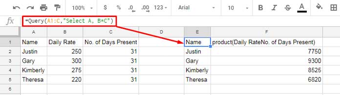
Addition in Google Sheets QUERY
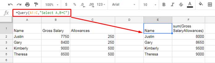
The following formula adds the values in columns B and C.
=QUERY(A1:C,"SELECT A, B + C")For example, if column B contains the basic salary and column C contains the allowance, the formula returns the total salary.
Subtraction in Google Sheets QUERY
In this example, column C contains the total number of days in the month, while column D contains the number of days an employee was absent.
To calculate the number of days worked, subtract column D from column C.
=QUERY(A1:D,"SELECT A, B, C - D")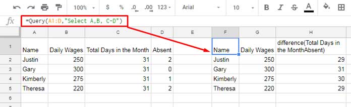
Division in Google Sheets QUERY
Suppose column B contains the quantity purchased and column C contains the total cost. To calculate the cost per unit, divide the total cost by the quantity.
=QUERY(A1:C,"SELECT A, C / B")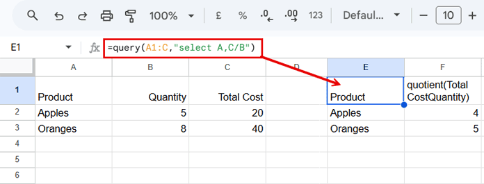
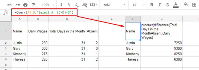
Using Multiple Arithmetic Operators
You aren’t limited to using a single arithmetic operator in a QUERY formula. You can combine multiple operators to perform more complex row-level calculations.
For example, suppose you want to calculate an employee’s gross wages using this formula:
Gross Wage = (Total Days in the Month − Absent Days) × Daily Wage
You can do that with the following QUERY formula:
=QUERY(A1:D,"SELECT A, (C - D) * B")In this example, the expression (C - D) calculates the number of days worked, and the result is then multiplied by the daily wage in column B.
Note: Arithmetic expressions in QUERY follow the standard order of operations. Multiplication and division are evaluated before addition and subtraction. Use parentheses to override the default precedence.
Arithmetic with Aggregate Functions and GROUP BY
So far, we’ve used arithmetic operators for row-level calculations in the QUERY function. However, QUERY isn’t required for these calculations—you can often use regular spreadsheet formulas instead.
For example, to calculate the cost per unit for each row, you can simply use:
=LET(f, ARRAYFORMULA(IFERROR(C2:C/B2:B)), f)The real power of arithmetic operators in QUERY comes from combining them with aggregate functions such as SUM, AVG, COUNT, MIN, and MAX, especially when using a GROUP BY clause.
Let’s look at an example.
Suppose you have a dataset containing the date of supply, product name, number of trucks dispatched, and number of rejected truckloads.
To calculate the actual number of trucks shipped for each product, subtract the rejected truckloads (column D) from the dispatched truckloads (column C), and then group the results by product (column B).
The following QUERY formula does exactly that:
=QUERY(A1:D,"SELECT B, SUM(C)-SUM(D) WHERE B IS NOT NULL GROUP BY B")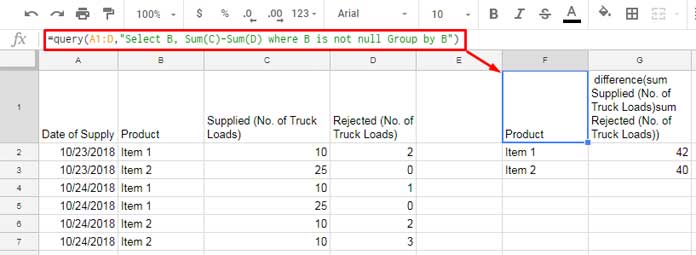
Now let’s extend this example.
Assume each truck carries 45 cubic meters of material. You can convert the net number of trucks into the total quantity shipped (in cubic meters) by multiplying the result by 45.
=QUERY(A1:D,"SELECT B, (SUM(C)-SUM(D))*45 WHERE B IS NOT NULL GROUP BY B")Returning Both the Net Truck Count and Quantity
You might expect the following formula to return both the net number of trucks and the equivalent quantity in cubic meters:
=QUERY(A1:D,"SELECT B, SUM(C)-SUM(D), (SUM(C)-SUM(D))*45 WHERE B IS NOT NULL GROUP BY B")Since the SELECT clause cannot reuse the result of another calculated column, you must repeat the expression or calculate it in an inner QUERY first.
A simple workaround is to use a nested QUERY. The inner QUERY calculates the net truck count, and the outer QUERY converts it to cubic meters.
=QUERY(
  QUERY(A1:D,"SELECT B, SUM(C)-SUM(D) WHERE B IS NOT NULL GROUP BY B"),
  "SELECT Col1, Col2, Col2*45"
)
This returns both the net truck count and the quantity in cubic meters side by side.
How to Rename (Label) Calculated Columns
When you use arithmetic operators in the QUERY function, the calculated columns are assigned default labels. These labels are often long or difficult to read because they’re generated from the expression itself.
You can replace the default label with a more meaningful one by using the LABEL clause.
For example, consider the following formula:
=QUERY(A1:C,"SELECT A, B * C")The calculated column is assigned a default label similar to:
B * C
(or product(BC), depending on the type of expression and your data).
To replace it with a more descriptive label, such as Monthly Pay, use the LABEL clause:
=QUERY(A1:C,"SELECT A, B * C LABEL B * C 'Monthly Pay'")The output column will now be labeled Monthly Pay instead of the default expression.
FAQ
Can I use arithmetic operators with SUM() in QUERY?
Yes. You can combine arithmetic operators with aggregate functions such as SUM(), AVG(), COUNT(), MIN(), and MAX(). This is especially useful when using a GROUP BY clause.
Does QUERY support parentheses in arithmetic expressions?
Yes. You can use parentheses to control the order of operations and override the default arithmetic precedence.
Why does my arithmetic QUERY return #N/A?
This usually happens because the SELECT clause cannot reuse the result of another calculated expression. Use a nested QUERY if you need to reference a calculated value in another expression.
Can I rename calculated columns?
Yes. Use the LABEL clause to assign a custom name to a calculated column instead of the default label.
Conclusion
Arithmetic operators let you perform calculations directly within the QUERY function without adding helper columns. While they’re useful for simple row-level calculations, they become especially powerful when combined with aggregate functions and clauses such as GROUP BY, WHERE, and ORDER BY. By using arithmetic expressions together with the LABEL clause and nested QUERY formulas when needed, you can build more compact and flexible queries.


Hi Prashant
Thank you so much for sharing this. It’s immensely helpful articles.
Question: Whats the power operator (exponent operator) inside the query? I tried using “^”, “**” but neither works? Please suggest
=Query({A1:A50}, "select Col1^2")Hi, Chan,
As far as I know, such use is not supported in Query. So try to use it as below.
=ArrayFormula(Query(if(len(A2:A),A2:A^2,), "select Col1"))I have started the range from A2 instead of A1 considering the title in A1.
Can I use round in google sheets query? if Yes how?
Like if a 3/10 it gives me 0 instead of 0.3
and 12/10 it gives me 1 instead of 1.2
and 23/10 it gives me 2 instead of 2.3
How can this be done in google sheets query?
Hi Prashanth,
I hope you’re doing great. Infinite thanks for all the different articles you’ve done so far. It has helped me a couple of times!
I’ve got a question about query multiplication and I’m not sure there is an easy fix to that…
You’ve 2 columns with numbers and some raws from 1 column have empty cells. If I do the Query, there is going to be empty raws where there are only 1 number (it looks like that Google Sheets Query doesn’t multiply a cell with an empty cell).
Any thoughts about that would be very appreciated 🙂
Thanks, & take care!
Dimitri
Hi, Dimitri,
Assume the columns are A and B, and A1:1 (first row) contains headers.
Then you may try it.
=query(query(A2:B,"Select * where A*B is not null",0),"Select Col1,Col2,Col1*Col2",0)It would return the result in three columns – Colum A values, Column B values, and the multiplication result. There won’t be any blank row in the output.
Hey Prashanth 🙂
Thanks for this quick answer! I’m very pleased to read from you. One thing I noticed when I saw your solution is that I forgot to mention my need to keep those numbers that have empty cells in front of (like if they were multiplied by 1). Visual explanation : (desired result in column C)
A|B|C
2|14|28
3|7|21
4|4
So far, and after reading your blog I’m using the
N()function. That looks like this (let’s consider that empty cells appear only in column B):=Query({Query({A:B},"Select Col1",1),ArrayFormula(N(Query({A:B},"Select Col2",1))+1)},"Select Col1*Col2",1)
Is there any easiest way to find the same solution?
Thanks again!
Best
Edit: I can see for the visual explanation that spaces between letters have been cropped. On the 4th line, the second number “4” belongs to column C
🙂
Hi, Dimitri Leroux,
Now I could understand what you are trying to do.
Here are my formulas. Row#1, i.e. A1:B1, contains headers. So I am not considering it in my formula. I would select A2:B.
Formula without using Query but using arithmetic and comparison operators in cell C1:
={"Product";ArrayFormula(if(A2:A+B2:B>0,if(A2:A="",1,A2:A)*if(B2:B="",1,B2:B),))}Or you can use the below Query in cell C1:
=Query(ArrayFormula(if(A2:A+B2:B>0,{if(A2:A="",1,A2:A),if(B2:B="",1,B2:B)},)),"Select Col1*Col2")From my test your formula is not working properly.
Hey Prashanth,
Thanks so much for all of this! I never even knew about the Query!
I’m having a little trouble with combining things from different tabs and I’m not sure what I’m doing wrong. I’d be happy to attach screen shots if you want to e-mail me, but basically:
Row 1 is the header
Column A contains names, some of which are repeating ex:
Tom
Larry
Cindy
Tom
Mary
Cindy
Tom
Columns B-H are different stats for each person, such as wins, loss, ties, etc. but from different seasons.
So I’m basically trying to consolidate to only have 1 of each name, and add their stats so each name has 1 row with all of their stats across B-H, hoping this would enable me to rank based on total numbers.
I was taking all of the information from tab 2 and trying to consolidate on tab 1, but I can’t seem to figure out what the formula is supposed to be for everything. Hope this all makes sense, and thanks in advance.
Hi, Alex,
If your data is in ‘Sheet1’, in Sheet2 (or any other sheet) use this formula.
=query(Sheet1!A1:H,"Select A, sum(B),sum(C),sum(D),sum(E),sum(F),sum(G),sum(H) where A is not null group by A",1)If it doesn’t work try changing the first and last comma to semicolon as per regioinal settings.
Also, you can share with me a demo sheet.
Hi,
My query is outputting a column with dates. Now I want to reduce each date by one day in the same column. For example, if the date is 06/29/2019, I want it to show 06/28/2019 using mathematical operators within the query function. Any ideas?
Hi, Varun,
See a similar topic: How to Add or Subtract N Days to The Dates in a Column in Sheets Query.
Best,
What if you wanted to query another sheet but add a calculation using data from the current sheet?
Hi, Cory,
Here is one example.
=Query({A1:B,Sheet1!C1:C},"Select Col1, Col2*Col3")