Want to add or subtract days from a date column using a QUERY formula in Google Sheets? Unfortunately, QUERY doesn’t support direct date math—but don’t worry! In this guide, I’ll show you two simple workarounds to add or subtract N days from dates within a QUERY, whether you’re calculating expiry dates, filtering task deadlines, or performing any kind of time-based logic.
This tutorial is part of the Date Logic in QUERY hub.
Learn how date logic works in Google Sheets QUERY, including date criteria, month-based filtering, and DateTime handling.
Why Regular Date Math Doesn’t Work in QUERY
Let’s say you want to add 30 days to dates in column B using this formula:
=QUERY(A1:C, "SELECT B+30")This won’t work. You’ll see a #VALUE! error:
“Can’t perform the function SUM on values that are not numbers.”
Now let’s try subtracting 30 days:
=QUERY(A1:C, "SELECT B-30")Same issue. QUERY doesn’t perform arithmetic on date-type columns directly.
So, how do we work around this?
2 Ways to Add or Subtract Days from Dates in a QUERY Formula
Method 1: Convert Dates to Numbers First
Dates in Google Sheets are stored as serial numbers (e.g., Dec 30, 1899 = 0). If we convert the dates to number format first, we can perform arithmetic in QUERY.
Example Data:
| A | B |
|---|---|
| Description | Purchase Date |
| Hosting 1 | 27/01/2019 |
| Domain Registration 1 | 27/01/2019 |
| Hosting 2 | 14/06/2019 |
| Domain Registration 2 | 14/06/2019 |
Steps:
- Select column B → Format → Number → Number.
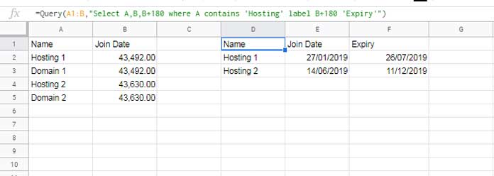
- Use this formula to add 180 days:
=QUERY(A1:B, "SELECT A, B, B+180 WHERE A CONTAINS 'Hosting' LABEL B+180 'Expiry'")Don’t forget to format the output columns back to date using Format → Number → Date.
Method 2: Use DATEVALUE with ArrayFormula
This method lets you keep column B as actual dates and handle the conversion inside the formula.
=ARRAYFORMULA(QUERY({A1:A, DATEVALUE(B1:B)},
  "SELECT Col1, Col2, Col2+180 WHERE Col1 CONTAINS 'Hosting' LABEL Col2+180 'Expiry'"))
👉 When using expressions on query data created using array literals, always refer to columns as Col1, Col2, etc., instead of A, B, etc.
Dealing with Header Errors
If your data includes headers, DATEVALUE will throw an error on the text in row 1. To fix this, just add a second label to rename the second column:
=ARRAYFORMULA(QUERY({A1:A, DATEVALUE(B1:B)},
  "SELECT Col1, Col2, Col2+180 WHERE Col1 CONTAINS 'Hosting' LABEL Col2 'Join Date', Col2+180 'Expiry'"))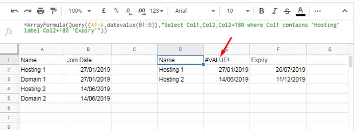
How to Subtract Days from Dates in QUERY
To subtract instead of add, simply replace + with -.
Method 1 (Using Converted Numbers):
=QUERY(A1:A, "SELECT A, A-30")Format output column as a date.
Method 2 (Using DATEVALUE):
=ARRAYFORMULA(QUERY(DATEVALUE(A1:A),
  "SELECT Col1, Col1-30 LABEL Col1 'Date', Col1-30 'Date-30'"))
Again, format the output columns as dates.
Conclusion
That’s it! Now you know how to add or subtract days from dates in a column using a QUERY in Google Sheets. Whether you prefer formatting your source column or using DATEVALUE inside an ARRAYFORMULA, these two methods help you work around the date arithmetic limitation in QUERY.


Thanks, I got the output for the above ask.
Thanks, Prashanth,
How do we change the date by adding time to it?
Example: The Planned start time is 23:50:00 PM and Planned end time is 3:20:00 AM
The Planned start date is 8/7/2019 and how to get the planned output basis on 3 conditions?
I need output as next day date (8/8/2019) after adding start and end time to the current date.
Hi,
How to add or subtract 1 hour when between two times exceed 9 hours?
Example: If we add 9 hours to start time 10:00:00 AM then the output should roundup to 8 hours only (18:00:00)
Hi, Hima,
Assume the following values are present in your Sheet.
Cell B2: 10:00:00 – This is in time format
Cell C2: 10 – this is hours as a number.
Formula to be used in cell D2 to conditionally add hours to time.
=if(C2>8,B2+time(8,0,0),B2+time(C2,0,0))Best,