Group and Sum Time Duration Using Query in Google Sheets (2 Easy Methods)

If you’re looking to group and sum time duration using Query in Google Sheets, you’re in the right place. In this post, I’ll show you two different methods to do just that.

One method is simpler but requires manual formatting, while the other is fully automated using formulas only.

Let’s explore both options — and also learn how to fix the common #VALUE! error when using the SUM function with time durations in a Google Sheets QUERY.

Why Query SUM Returns an Error with Time Duration

If you try to use the QUERY function to sum a time duration column directly, like this:

=QUERY(A1:E, "SELECT SUM(E)", 1)

You’ll likely get a #VALUE! error.

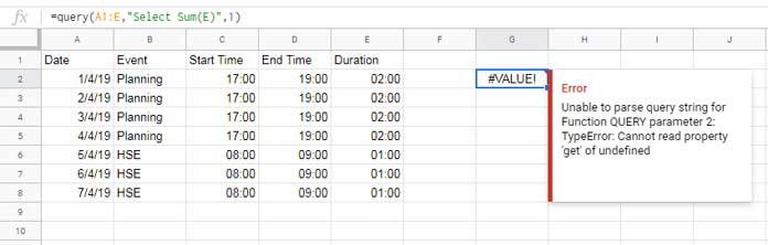
Google Sheets QUERY returns error when using time duration in aggregation with SUM function

As shown in the screenshot, the error occurs because Google Sheets expects numeric values for aggregation. The tooltip indicates:
“AVG_SUM_ONLY_NUMERIC”, meaning the column contains non-numeric data (in this case, durations formatted as time).

So before you can group and sum time duration using Query, you need to convert those time values to numeric format.

Method 1: Sum Time Duration Using Query + Manual Formatting

This is the simplest method if you don’t mind applying some manual formatting.

Step 1: Convert Duration Format

Select the range E2:E (your Duration column), go to the Format menu, and choose: Format > Number > Number

Now you can use this formula:

=QUERY(A1:E, "SELECT SUM(E)", 1)

But the result will appear as a decimal number. To convert it back to time format, select the result cell and go to: Format > Number > Duration

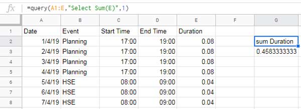
Alternatively, apply the formatting directly within the formula like this:

=QUERY(A1:E, "SELECT SUM(E) FORMAT SUM(E) '[h]:mm:ss'", 1)

That’s it! You’ve now learned to sum time duration using Query with minimal effort.

Method 2: Query Formula Without Manual Formatting

If you prefer not to change the format manually, here’s a formula-only method.

Step 1: Convert Duration to Numeric Using `N`

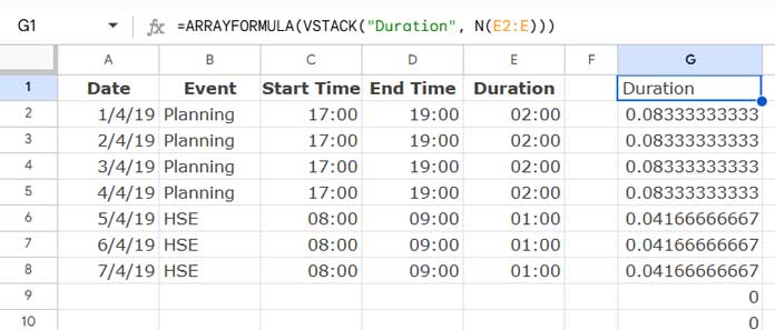
Wrap your Duration column in an ARRAYFORMULA using the N() function:

=ARRAYFORMULA(VSTACK("Duration", N(E2:E)))

This converts the time durations to numbers. VSTACK is used to include the header.

Example showing how to convert duration to numeric format for use in Google Sheets QUERY function

Step 2: Combine with Original Data Using `HSTACK`

Now, stack this new numeric Duration column next to your existing data:

=HSTACK(A1:D, ARRAYFORMULA(VSTACK("Duration", N(E2:E))))

Use this as the input range in your query:

=QUERY(HSTACK(A1:D, ARRAYFORMULA(VSTACK("Duration", N(E2:E)))), "SELECT SUM(Col5) FORMAT SUM(Col5) '[h]:mm:ss'", 1)

Note: When using virtual ranges like this, you must reference columns by number (e.g., Col5), not letter (e.g., E).

How to Group and Sum Time Duration Using Query

Once you’ve converted your durations correctly, grouping them is straightforward. Here’s how to group and sum time duration using Query based on a specific column — such as “Event”.

Method 1: Grouping with Manual Formatting

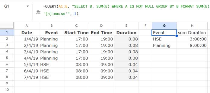
First, ensure column E is formatted as Number, then use:

=QUERY(A1:E, "SELECT B, SUM(E) WHERE A IS NOT NULL GROUP BY B FORMAT SUM(E) '[h]:mm:ss'", 1)

Result:

Example of how to group and sum time duration using the QUERY function in Google Sheets

Method 2: Grouping Without Manual Formatting

You can also group using the virtual range:

=QUERY(HSTACK(A1:D, ARRAYFORMULA(VSTACK("Duration", N(E2:E)))), "SELECT Col2, SUM(Col5) WHERE Col1 IS NOT NULL GROUP BY Col2 FORMAT SUM(Col5) '[h]:mm:ss'", 1)

This groups the events in column B (Col2) and sums the corresponding durations (Col5), all without manual formatting.

Conclusion

Whether you prefer a simple solution with minor formatting or a formula-only approach, you now know how to group and sum time duration using Query in Google Sheets. Both methods are flexible and powerful depending on your needs.

Resources

Hi, Sara,

First, let me answer your question number 2.

Question 2:

The use of 0 or 1 is actually to specify whether there is a header row (a row with labels) in your selected range. 0 represents 0 label row, 1 represents 1 label row, 2 represents two label rows and so on.

Query Syntax:

QUERY(data, query, [headers])

Actually, the headers is an optional argument in Query. If you exclude specifying headers, Query will automatically detect the headers.

Question 1:

It’s regarding the use of backslash. If you have checked my article (link shared on my previous reply) regarding how to convert nonregional formulas (formula locale settings), you could understand this usage.

Depending on your region, you may want to replace a , in my formula with ; as the separator within a function. As far as I know in most of the EU countries ; replaces , as the separator.

Then your question is why I have replaced a , in the first part of the Query with \.

The answer is within curly brackets, the , should be replaced with a \ not a ;

Best,

15 COMMENTS

Sara Polselli November 5, 2019 At 3:11 am

Hi Prashanth,

Thanks a lot.

Here it is:

Link copied, then removed – Admin.

I hope I’ve shared it correctly.

Thanks.
.S.

- Prashanth November 7, 2019 At 9:04 am
  
  Hi, Sara,
  
  Sorry for the late reply. I was offline for two days.
  
  Now to your problem.
  
  I could find two issues.
  
  1. Your sample data is in the ottobre tab and the formula is in another tab. So in the formula correctly refer to the source. The range used in your formula is ottobre!A1:C and D1:D. You have missed ottobre! with D1:D.
  
  2. You may please see my formula. I have used the duration column range from the second row skipping header. So you should use ottobre!D2:D instead of D1:D.
  
  So the formula would be;
  
  =Query({ottobre!A1:C\{"per progetto - OTTOBRE";ArrayFormula(if(len(ottobre!D2:D);(hour(ottobre!D2:D)/24+minute(ottobre!D2:D)/1440+second(ottobre!D2:D)/86400);))}};"Select Col1,Sum(Col4) where Col1 is not null group by Col1 format Sum(Col4) 'HH:MM:SS'";1)
  
  Note for other readers: This formula is for Italian locale.
  
  Best,
  
  - Sara Polselli November 7, 2019 At 6:31 pm
    
    Hi Prashanth,
    
    I must admit I’m rather ashamed, I changed the reference to only the first occurrence… sorry for disturbing you for what I could have done on my own with some more care. Thanks anyway!
    
    Only one further question: why do I have to manually set the Format of the duration column to Duration? If I don’t do that then I get times instead but I thought that the format Sum(Col4) ‘HH:MM:SS’ part of the formula meant to spare having to set the format manually. Am I wrong?
    
    Thanks for your time and patience.
    .S.
    
Sara Polselli November 3, 2019 At 8:23 pm

Hi Prashanth,

Sorry to bother you again, I’m not sure you can give me some hints on this.

I would now like to reference a data set on another sheet of the same spreadsheet so as to use a sheet for the data and another for the queries. I have done it on another spreadsheet and other data and it worked but on this, I get a #REF! error.

My formula is:

=Query({'Produzione AGOSTO'!A1:C\{"per progetto - AGOSTO";ArrayFormula(if(len(D1:D);(hour(D1:D)/24+minute(D1:D)/1440+second(D1:D)/86400);))}};"Select Col1,Sum(Col4) where Col1 is not null group by Col1 format Sum(Col4) 'HH:MM:SS'";1)

and Produzione AGOSTO is the name of the sheet inside the spreadsheet.

The message I get related to the error is:

“Error”
“Function ARRAY_ROW parameter 2 has a mismatched row size. Expected: 999. Actual: 1001.”

I looked around on the internet but couldn’t find a solution. Should I share my spreadsheet with you?

Thanks!!

.S.

- Prashanth November 4, 2019 At 1:20 pm
  
  Hi, Sara,
  
  Feel free to share a copy of the concerned Sheet with me. I will definitely try to solve the problem as early as possible.
  
  Best,
  
Sara Polselli October 8, 2019 At 1:31 am

Hey, thanks a lot Prashanth, it works!

Thanks for pointing me out to the other article, I understand I should have changed all , into ; to adjust to my locale.

There are a couple of things I haven’t got clear and I would really appreciate if you’d be so kind as to explain to me.
1. Query({A1:C\{ : why is there a backslash in the range? Also: why the range doesn’t have to extend enough to include the column I want to sum?

2. Is the final ;0) or ;1) accounting for the no first row of labels vs yes the first row of labels?

Thanks again! Really!

.S.

- Prashanth October 8, 2019 At 9:50 am
  
  Hi, Sara,
  
  First, let me answer your question number 2.
  
  Question 2:
  
  The use of 0 or 1 is actually to specify whether there is a header row (a row with labels) in your selected range. 0 represents 0 label row, 1 represents 1 label row, 2 represents two label rows and so on.
  
  Query Syntax:
  
  QUERY(data, query, [headers])
  
  Actually, the headers is an optional argument in Query. If you exclude specifying headers, Query will automatically detect the headers.
  
  Question 1:
  
  It’s regarding the use of backslash. If you have checked my article (link shared on my previous reply) regarding how to convert nonregional formulas (formula locale settings), you could understand this usage.
  
  Depending on your region, you may want to replace a , in my formula with ; as the separator within a function. As far as I know in most of the EU countries ; replaces , as the separator.
  
  Then your question is why I have replaced a , in the first part of the Query with \.
  
  The answer is within curly brackets, the , should be replaced with a \ not a ;
  
  Best,
  
  - Sara Polselli October 8, 2019 At 5:59 pm
    
    Thanks.
    
    I had understood the ; vs , part of the article but I hadn’t clear about the use of \ replacing , inside {}. Now I know, thanks.
    
    .S.
    
  - Sara Polselli October 9, 2019 At 2:43 am
    
    Hi Prashanth,
    
    Thanks for your reply and for sharing the example datasheet with me.
    
    I figured out the problem with the sum I had: the format of the column containing the sum would go to “Automatic” and it would be interpreted as Time instead of Duration, so it would show me 15:30 (time) instead of 39.30 (duration).
    
    Once I selected Duration as the format of the Column containing the sum the numbers showed added up correctly.
    
    Best,
    
    .S.
    
Sara Polselli October 5, 2019 At 10:43 pm

Hi there.

Thanks for the article, it’s very clear and is exactly what I need: However, I can’t make the formula to work: it gives me a #ERROR! with a generic Formula parse error message.

Here is my formula

=Query({A1:D,{"Duration";ArrayFormula(if(len(D1:D),(hour(D1:D)/24+minute(D1:D)/1440+second(D1:D)/86400),))}},"Select Col1,Sum(Col4) where Col1 is not null group by Col1 format Sum(Col4) 'HH:MM:SS'",1)

where the Duration values I want to add are in Column D.

Any help you may give me? Thanks!!

- Prashanth October 6, 2019 At 8:39 am
  
  Hi, Sara,
  
  Can your Share your ‘Locale’ which you can find under your File menu Spreadsheet settings. Also, I want to know the following;
  
  1. The number of columns in your dataset.
  2. Whether the first row contains column names (field labels).
  3. Values in each column. I mean the column contains text, date, or time.
  
  Best,
  
  - Sara Polselli October 6, 2019 At 8:20 pm
    
    Hi Prashanth,
    
    Thanks for your reply!
    
    My “Locale” is Italy.
    
    As to replies to your questions:
    
    1. My dataset has 5 columns
    
    2. The dataset I’m working with is a test dataset and doesn’t have field labels. The one I will be interested in applying the formula to will have field labels in the first row.
    
    3. The first 3 columns contain text (data fed by another sheet). The 4th contains Duration (and it’s the one I want to add the values of). The 5th column contains a Date.
    
    Also, if I follow your option n. 1, with manual formatting, it works and I get the results I need. But it would be better for me and my team to be able to apply a formula that works always.
    
    Thanks!
    
    - Prashanth October 7, 2019 At 9:44 am
      
      Hi, Sara,
      
      My original formula after converting to your Locale.
      
      =Query({A1:D\{"Duration";ArrayFormula(if(len(E2:E);(hour(E2:E)/24+minute(E2:E)/1440+second(E2:E)/86400);))}};"Select Col2,Sum(Col5) where Col1 is not null group by Col2 format Sum(Col5) 'HH:MM:SS'";1)
      
      The same formula tuned for your dataset (for the fourth column as the ‘Duration’ column).
      
      First Row Contains Labels:
      
      =Query({A1:C\{"Duration";ArrayFormula(if(len(D2:D);(hour(D2:D)/24+minute(D2:D)/1440+second(D2:D)/86400);))}};"Select Col1,Sum(Col4) where Col1 is not null group by Col1 format Sum(Col4) 'HH:MM:SS'";1)
      
      The first Row Doesn’t Contain Labels:
      
      =Query({A1:C\{ArrayFormula(if(len(D1:D);(hour(D1:D)/24+minute(D1:D)/1440+second(D1:D)/86400);))}};"Select Col1,Sum(Col4) where Col1 is not null group by Col1 format Sum(Col4) 'HH:MM:SS'";0)
      
      This will work for you. If not, please let me know, I will share my Sheet with you.
      
      Also, please read – How to Change a Non-Regional Google Sheets Formula.
      
      Best,
      
      - Sara Polselli October 8, 2019 At 1:52 am
        
        Sorry, I misplaced my previous reply and it probably makes the thread hard to follow 🙁
        
        Anyway, I have a problem. The first row is calculated erroneously at first. It did go right after some time or some change I made but I can’t figure out why just the numbers didn’t add up to the correct value whereas afterward they mysteriously did.
        
        This, in my test dataset. In my real one, again, numbers don’t add up correctly. Any ideas why?
        
        Thanks!
        
        
        Prashanth October 8, 2019 At 10:00 am
        
        Hi, Sara,
        
        I think it’s high time to share a demo Sheet with you! I have set the locale to Italy.
        
        https://docs.google.com/spreadsheets/d/1BpL1PdACg74KrzIIc-JO71apEB1n1Iq7eqgWKR4Wvgs/copy
        
        See if that helps?
        
        Best,