How to Use SUM, AVG, COUNT, MIN, and MAX in Google Sheets QUERY

Aggregation functions in Google Sheets QUERY allow you to summarize data using SUM, AVG, COUNT, MIN, and MAX across one or more columns. This guide explains how each aggregation function works using clear formulas and result tables.

Google Sheets QUERY supports five aggregation functions:

SUM() – adds numeric values
AVG() – calculates the average
COUNT() – counts non-empty values in a column
MIN() – returns the smallest value
MAX() – returns the largest value

In this guide, you’ll learn how to use all five aggregation functions in Google Sheets QUERY, including:

Single-column and multi-column aggregations
Conditional aggregation using WHERE
Grouped aggregation using GROUP BY
QUERY-based alternatives to SUMIF, COUNTIF, AVERAGEIF, MINIFS, and MAXIFS

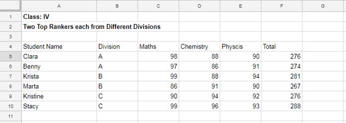
All examples in this tutorial use the same sample dataset (shown below), making it easy to compare how each aggregation function behaves across different scenarios.

Table of Contents

Sample Data

⚠️ Important: Google Sheets QUERY expects consistent data types within each column. Avoid using columns that contain mixed values (numbers and text), as this can lead to incorrect or unexpected results with aggregation functions such as SUM, AVG, COUNT, MIN, and MAX.

Example Sheet:

Copy Sample Sheet

This view-only Google Sheet contains the same sample data used throughout this tutorial. You can copy it to test all QUERY aggregation examples.

1. How to Use the SUM Function in Google Sheets QUERY

All examples below use the same sample data. Once you understand how SUM() works, you can easily apply the same logic to AVG(), COUNT(), MIN(), and MAX().

SUM() – Multiple Columns

Problem: Sum multiple numeric columns using QUERY.

=QUERY(A4:F,"select sum(C), sum(D), sum(E), sum(F)",1)

Result:

sum Maths	sum Chemistry	sum Physics	sum Total
569	543	550	1662

SUM() – Single Column

=QUERY(A4:F,"select sum(C)",1)

Explanation: This formula returns the total of all numeric values in column C (Maths).

Conditional SUM() – Single Column

Problem: Sum column C only where column B equals "C".

=QUERY(A4:F,"select sum(C) where B='C'",1)

Equivalent worksheet function:

=SUMIF(B4:B,"C",C4:C)

Note: SUMIF is not case-sensitive, while QUERY conditions are case-sensitive.

Conditional SUM() – Multiple Columns

=QUERY(A4:F,"select sum(C), sum(D), sum(E), sum(F) where B='C'",1)

Group and SUM()

=QUERY(
 A4:F,
 "select B, sum(C), sum(D), sum(E), sum(F)
  where A is not null
  group by B",
 1
)

Result:

Division	sum Maths	sum Chemistry	sum Physics	sum Total
A	195	174	181	550
B	185	179	184	548
C	189	190	185	564

Explanation:

Column B is grouped
All numeric columns are summed
Blank rows are excluded using A is not null

👉 In many cases, SUM() in QUERY can replace SUM, SUMIF, and SUMIFS.

2. How to Use the AVG Function in Google Sheets QUERY

The AVG() aggregation function works exactly like SUM(). You only need to replace SUM with AVG.

AVG() – Multiple Columns

=QUERY(A4:F,"select avg(C), avg(D), avg(E), avg(F)",1)

Result:

avg Maths	avg Chemistry	avg Physics	avg Total
94.83	90.5	91.67	277

AVG() – Single Column

=QUERY(A4:F,"select avg(C)",1)

Equivalent to the AVERAGE worksheet function.

Conditional AVG() – Single Column

=QUERY(A4:F,"select avg(C) where B='C'",1)

Equivalent worksheet function:

=AVERAGEIF(B4:B,"C",C4:C)

Conditional AVG() – Multiple Columns

=QUERY(A4:F,"select avg(C), avg(D), avg(E), avg(F) where B='C'",1)

Group and AVG()

=QUERY(
 A4:F,
 "select B, avg(C), avg(D), avg(E), avg(F)
  where A is not null
  group by B",
 1
)

Result:

Division	avg Maths	avg Chemistry	avg Physics	avg Total
A	97.5	87	90.5	275
B	92.5	89.5	92	274
C	94.5	95	92.5	282

3. How to Use the COUNT Function in Google Sheets QUERY

The COUNT() aggregation function in QUERY counts non-empty values in the selected column, including both numbers and text.

COUNT() – Multiple Columns

=QUERY(A4:F,"select count(C), count(D), count(E), count(F)",1)

Result:

count Maths	count Chemistry	count Physics	count Total
6	6	6	6

COUNT() – Single Column

=QUERY(A4:F,"select count(C)",1)

Conditional COUNT() – Single Column

=QUERY(A4:F,"select count(C) where B='C'",1)

Equivalent worksheet function:

=COUNTIF(B4:B,"C")

Conditional COUNT() – Multiple Columns

=QUERY(A4:F,"select count(C), count(D), count(E), count(F) where B='C'",1)

Group and COUNT()

=QUERY(
 A4:F,
 "select B, count(C), count(D), count(E), count(F)
  where A is not null
  group by B",
 1
)

Result:

Division	count Maths	count Chemistry	count Physics	count Total
A	2	2	2	2
B	2	2	2	2
C	2	2	2	2

Important:

When used with GROUP BY, COUNT() returns the number of non-empty values per group, which effectively represents the number of rows when the counted column is populated.

To calculate metrics such as unique products per day or distinct items per category, you must remove duplicates first (for example, using UNIQUE()), and then apply COUNT() on the deduplicated result.

👉 See the dedicated guide on counting unique values in Google Sheets QUERY, which demonstrates how to combine UNIQUE() with QUERY() using real-world examples with date, item, and quantity columns.

4. How to Use the MIN Function in Google Sheets QUERY

The MIN() aggregation function returns the smallest numeric value.

MIN() – Multiple Columns

=QUERY(A4:F,"select min(C), min(D), min(E), min(F)",1)

Result:

min Maths	min Chemistry	min Physics	min Total
86	86	90	267

MIN() – Single Column

=QUERY(A4:F,"select min(C)",1)

Conditional MIN() – Single Column

=QUERY(A4:F,"select min(C) where B='C'",1)

Equivalent worksheet function:

=MINIFS(C4:C, B4:B, "C")

Conditional MIN() – Multiple Columns

=QUERY(A4:F,"select min(C), min(D), min(E), min(F) where B='C'",1)

Group and MIN()

=QUERY(
 A4:F,
 "select B, min(C), min(D), min(E), min(F)
  where A is not null
  group by B",
 1
)

Result:

Division	min Maths	min Chemistry	min Physics	min Total
A	97	86	90	274
B	86	88	90	267
C	90	94	92	276

5. How to Use the MAX Function in Google Sheets QUERY

The MAX() aggregation function returns the largest numeric value.

MAX() – Multiple Columns

=QUERY(A4:F,"select max(C), max(D), max(E), max(F)",1)

Result:

max Maths	max Chemistry	max Physics	max Total
99	96	94	288

MAX() – Single Column

=QUERY(A4:F,"select max(C)",1)

Conditional MAX() – Single Column

=QUERY(A4:F,"select max(C) where B='C'",1)

Equivalent worksheet function:

=MAXIFS(C4:C, B4:B, "C")

Conditional MAX() – Multiple Columns

=QUERY(A4:F,"select max(C), max(D), max(E), max(F) where B='C'",1)

Group and MAX()

=QUERY(
 A4:F,
 "select B, max(C), max(D), max(E), max(F)
  where A is not null
  group by B",
 1
)

Result:

Division	max Maths	max Chemistry	max Physics	max Total
A	98	88	91	276
B	99	91	94	281
C	99	96	93	288

Conclusion

This tutorial covered all five aggregation functions in Google Sheets QUERY: SUM, AVG, COUNT, MIN, and MAX.

Once you learn one aggregation function, the others become easy because they all follow the same QUERY structure—the function name is the only difference.

Aggregation functions make QUERY one of the most powerful tools for data analysis, reporting, and automation in Google Sheets.

24 COMMENTS

ali January 10, 2024 At 3:57 pm

Good day, I have a problem with the GOOGLEFINANCE command, and I came across your post while trying to solve it. I would be happy if you could help me.

In the spreadsheet, I am attempting to find the lowest price of stock market shares between a certain date:

=MIN(GOOGLEFINANCE(A4, "LOW", "01.09.2023", "29.12.2023"))

This formula works and gives the correct result.

However, when I try to find the highest price using:

=MAX(GOOGLEFINANCE(A4, "LOW", "01.09.2023", "29.12.2023"))

It returns a value like this: 45135.75694. I would appreciate it if you could assist me with this issue.

- Prashanth KV January 10, 2024 At 6:55 pm
  
  Hi Ali,
  
  Firstly, I recommend replacing “01.09.2023” with DATE(2023, 9, 1) and “29.12.2023” with DATE(2023, 12, 29) to avoid date formatting-related issues. However, these changes won’t address the problem with MAX.
  
  The value you see when using MAX is a timestamp in date value.
  
  You can use the following formula:
  
  =QUERY(GOOGLEFINANCE(A4,"LOW", DATE(2023, 9, 1), DATE(2023, 12, 29)), "select max(Col2) label max(Col2)''", 1)
  
  I hope that helps.
  
  - ali January 16, 2024 At 9:15 am
    
    When I enter the query into the spreadsheet, it returns an error due to a formula parsing issue.
    
    - Prashanth KV January 16, 2024 At 11:30 am
      
      Please feel free to share a copy of your sheet with the original data replaced by sample data.
      
      - ali January 19, 2024 At 8:30 am
        
        I have emailed the file to your email address.
        
        
        Prashanth KV January 19, 2024 At 9:08 am
        
        Already replied. The issue is with the function separator. You must use a semicolon “;” instead of a comma “,” in your formulas. I couldn’t edit your sheet as it was set to VIEW only.
        
Jason July 25, 2021 At 1:55 am

Hi,

Thank you for this great article!

Does the Query command support Countif in the select statement? I keep getting VALUE errors when trying to use it.

Let’s say I have a three-column table with StudentName, Division, and ActiveFlag where the ActiveFlag is either “Active” or “Inactive.”

I want the query results to have three output columns for Division, ActiveStudents, InactiveStudents, and total the number of students from each division for their respective status flags.

example input:
Name, Division, StatusFlag
Bob, A, Active
Joe, A, Inactive
Ann, B, Active
Sara, B, Inactive
John, A, Active

Example Output:
Division, ActiveStudents, InactiveStudents
A, 2, 1
B, 1, 1

I hope this makes sense. Thanks again for the article! Any help is greatly appreciated.

Cheers!

- Prashanth July 25, 2021 At 10:56 am
  
  Hi, Jason,
  
  Assume the data is in A2:C, and the first row takes the field labels (header row).
  If so, in cell E1, insert the below Query formula, which uses the Pivot clause.
  
  =query(A1:C,"Select B,count(A) where A is not null group by B pivot C",1)
  
  Related:- What is the Correct Clause Order in Google Sheets Query?
  
Thomas March 15, 2021 At 6:16 am

Hi,

I’m looking to do something similar to Ali except I am attempting to get a count instead of a sum. I switched around the suggestion you left:

=iferror(n(query(Energy_Efficiency!D2:F, "Select Count(D) where D='State' and F='Action Plan' label Count(D) ''")),0)

However, I’m now attempting to count all instances of a keyword, along the lines of something similar to

=Countif(Energy_Efficiency!I1:I, "*Action Plan*")

I’m running into the issue where Countif doesn’t allow (?) for more than arguments but the former iferror(n(query formula runs into an error using * and only returns 0.

Do you know of any workarounds? Sorry if this is unclear!

- Prashanth March 15, 2021 At 12:55 pm
  
  Hi, Thomas,
  
  You can use wildcards in COUNTIFS too.
  
  Eg.
  
  =COUNTIFS(Energy_Efficiency!D1:D,"State",Energy_Efficiency!F1:F, "*Action Plan*")
  
  If you are particular in using QUERY, you should use the CONTAINS substring match as below.
  
  =iferror(n(query(Energy_Efficiency!D2:F, "Select Count(D) where D='State' and F contains 'Action Plan' label Count(D) ''")),0)
  
Mike February 23, 2021 At 6:40 pm

Every time I add the AND SUM(G)>0 I get an error that the sum(g) can’t be part of a where clause. Col G contains both positive and negative numbers and I want to know the balance only if it’s positive. I hope my question makes sense?

- Prashanth February 24, 2021 At 10:16 am
  
  Hi, Mike,
  
  In a blank cell (eg. cell A1) get the total of column G. Then do a logical test as below.
  
  =if(A1<=0,,your_query_formula)
  
  If this doesn't help, if possible, reply with your (sample) sheet link.
  
Andrew Edwards September 23, 2020 At 4:44 am

Hi,

Love this article.

I’m trying to select the value (text) in column A based in the max value (numeric) in column B, there may be multiple max values and so I want to return each of them as a list.

I’m sure query is the way to do it and that the max() aggregation needs to be there but I can’t make it work.

I’ve tried;

Formula # 1

=QUERY(A1:B10,"select A where max(B)")

Formula # 2

=QUERY (A1:B10,"select A, max(B)")

and a couple of others besides. Any tips on getting this query to work.

Many thanks.

- Prashanth September 23, 2020 At 11:24 am
  
  Hi, Andrew Edwards,
  
  You can simply use the Filter function.
  
  =filter(A1:A10,B1:B10=max(B1:B10))
  
  If you want Query, use the MAX worksheet function within Query as below.
  
  =query(A1:B10,"Select A where B="&max(B1:B10))
  
Rob Weber May 22, 2020 At 8:50 pm

Hi there, I’m hoping someone can help me out.

I have a spreadsheet template from my office that I’d like to convert from excel to Google sheets so that I can have some data added automatically from a parsed source.

I have set this up, however, some of the formulas used in the original excel file are not able to be used in the sheets. Specifically I have a formula using aggregate functions. I cannot seem to figure out how to get this formula right in sheets.

This is the formula: =IFERROR(IF(AGGREGATE(3,5,[@[OUTSTANDING AMOUNT]])=1,1,0),"")

I need to rewrite this…I am assuming as a Query? Any assistance is greatly appreciated.

P.S. The @ aspect of the formula was added automatically by the new version of excel. I cannot seem to get it to show the original formula I had in that cell prior.

- Prashanth May 23, 2020 At 8:21 am
  
  Hi, Rob Weber,
  
  The Aggregate alternative is Subtotal, which is available in Google Sheets.
  
  If you can link to an example sheet, that contain your said problem and the expected output, I can try with Subtotal or Query.
  
Producer February 25, 2020 At 10:44 pm

Hello! I’m trying to create a query that grabs the hours worked from a separate sheet and then averages them to check for the average variance between hours estimated and actuals.

=SUM(QUERY(Test!$D:$K,"select K where D MATCHES '"&$B3&"'",0))

This allows me to total the actual hours worked that week.

=Average(QUERY(Test!$D:$J,"select J where D MATCHES '"&$B3&"'",0))

However, this gives me a DIV/0 error.

Any advice?

B3 is the name of the engineer who worked on the task. That name appears on both charts and I’m trying to do it this way so I don’t have to manually add tasks completed by the engineers.

- Prashanth February 26, 2020 At 9:10 am
  
  In the second Query did you use the column in the select clause correctly? I mean “select J” instead of “select K”?
  
  If that is not making the error, then I wish to see a demo of your dataset to suggest the cause or answer the problem.
  
ShirlyGirl February 21, 2020 At 5:14 pm

I have multiple boolean columns in my sheet. I’m trying to get a count of the number of times ‘true’ appears for each of the columns using a query (I was able to achieve it using COUNTIF formula directly in the sheet). Will any of these math functions help me achieve this via query?

- Prashanth February 21, 2020 At 7:35 pm
  
  Hi, ShirlyGirl,
  
  Multiply the range by 1 to convert TRUE to 1 and FALSE to 0. Then use the Query. Here is an example.
  
  =ArrayFormula(query(A1:C*1,"Select Sum(Col1),Sum(Col2),Sum(Col3)"))
  
Emerson Luiz Oliveira July 26, 2019 At 9:08 pm

Thanks a lot for the article!

One doubt: how can I eliminate the header that generates automatically? In the sum example, how can I display the result without showing Sum Math?

Once again, thanks a lot!

- Prashanth July 27, 2019 At 9:57 am
  
  Hi, Emerson,
  
  Use the Query Label clause. Here is one example to the use of Label caluse in Sum.
  
  =query(A4:F,"Select Sum(C),Sum(D),Sum(E),Sum(F) label Sum(C)'', Sum(D)'', Sum(E)'', Sum(F)''",1)
  
  To modify the label, I mean the sum Math, use this.
  
  =query(A4:F,"Select Sum(C),Sum(D),Sum(E),Sum(F) label Sum(C)'Maths', Sum(D)'Chemistry', Sum(E)'Physics', Sum(F)'Total'",1)
  
  Best,
  
Ali July 14, 2019 At 4:11 pm

Thanks a lot! Great article.

Have a question:

I’ve written a simple query to add up the sales we got from each lead, where the lead source is Facebook.
leads = a named range
AD = sale amount
L = lead source column

query(leads, " select sum(AD) where L = 'Facebook' label sum(AD) ''")

1. if there is at least 1 Facebook lead that has a sale, work correctly (eg. $3,000)
2. if there is at least 1 Facebook lead, but none of them had a sale, give #N/A
3. if there are no Facebook leads at all, then it returns empty cell

I want scenarios 2 & 3 to default to 0, but can’t figure it out with IFNA or IFERROR or anything else I’ve tried. Could you please help me out?!

Thank you so much <3

- Prashanth July 14, 2019 At 4:57 pm
  
  Hi, Ali,
  
  Try this Query. In this, the function N converts the blank to zero. The IFERROR converts the error value to zero.
  
  =iferror(n(query(leads, "select sum(AD) where L = 'Facebook' label sum(AD)''",1)),0)