This post describes how to filter out blank columns in Google Sheets using a combination formula that is easy to understand.
When we have blank columns, we usually delete or hide them. However, this may not be practical if the data is a formula expression, such as a VLOOKUP, QUERY, or IMPORTRANGE formula result.
In this walkthrough guide, we will discuss how to filter out blank columns in Google Sheets using formulas.
As a side note, we can use the FILTER or QUERY function to filter out blank rows. For example, the following formula will filter out all rows where column B is blank:
=QUERY(A1:B,"Select * Where A<>'' and B<>''")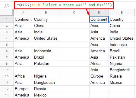
The Importance of Removing Empty Columns in Google Sheets
Blank columns can make your data look cluttered and unprofessional, and they can also make it difficult to analyze your data. By removing blank columns, you can make your data easier to read, understand, and print.
I have a Google Sheets spreadsheet with data in several rows and columns. Some of the columns in the table are completely blank.
I cannot predict which columns will be blank in the future, as the values in these columns are dynamic. This means that manually hiding the columns is not an ideal solution.
You can use a QUERY and FILTER combination formula to remove blank columns in Google Sheets. In this post, I will provide you with a dynamic formula that can cover all the rows in your data and several columns.
How to Filter Out Blank Columns in Google Sheets With a Header Row
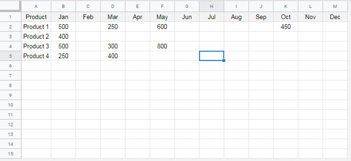
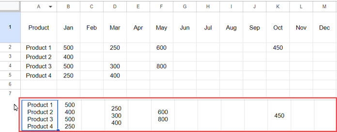
In the following spreadsheet (see screenshot below), I have a monthly breakdown of purchases for a few products in the tab Test Data, range A1:M. There are 13 columns in the table: a description column and 12 months columns.
In this table, I have values in the description column and the January, March, May, and October columns.
How do I extract only those columns that have at least one value other than the header?
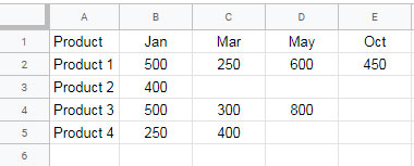
We can use the following FILTER + QUERY formula combination in another tab to filter out blank columns in Google Sheets when the header (title) row is present:
=FILTER('Test Data'!A1:M,LEN(TRIM(QUERY('Test Data'!A2:M,,9^9))))Where:
'Test Data'!A1:Mis the range reference of the table to filter, including the header row.'Test Data'!A2:Mis the criteria reference of the table to filter, excluding the header row.
This will populate the below output that doesn’t contain any empty columns!
Note: Please scroll down to see the formula explanation.
How to Filter Out Blank Columns in Google Sheets Without a Header Row
In our first example, we have a header row. So we need to exclude that while identifying the blank columns. We did that in the formula by specifying the filter range 'Test Data'!A1:M and criteria range 'Test Data'!A2:M.
I’ll explain how that formula works in more detail after seeing how to use QUERY with FILTER to remove or exclude blank columns in Google Sheets when no header row is present.
Sometimes we won’t use any header row, for example when entering some random data such as test results, or some ideas in sheets. For example, please see the below spreadsheet where data is spread across the Sheet in the range 'Test Data 2'!A1:Z.
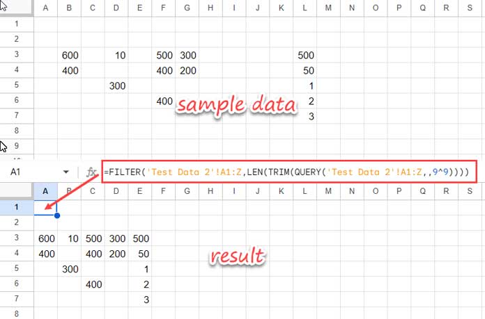
How to filter out all blank columns in Google Sheets using QUERY and FILTER when there is no header row?
We can use the first formula after making one change.
Instead of specifying different ranges for the FILTER and criteria arguments, we need to specify the same range for both arguments.
=FILTER('Test Data 2'!A1:Z,LEN(TRIM(QUERY('Test Data 2'!A1:Z,,9^9))))Where:
'Test Data 2'!A1:Zis the range reference of the table to filter, including or excluding the header row, depending on your needs.
Anatomy of the Formulas
We have seen two formulas to filter out blank columns: one for a table with a header row and one for a table without a header row.
I’ve already explained how to use them. Here is an explanation of the QUERY and FILTER functions in the formulas:
Syntax of the FILTER function:
FILTER(range, condition1, [condition2, …])In our first formula [ =FILTER('Test Data'!A1:M,LEN(TRIM(QUERY('Test Data'!A2:M,,9^9)))) ], the range is 'Test Data'!A1:M, and the condition1 is LEN(TRIM(QUERY('Test Data'!A2:M,,9^9))).
We just need to use the condition1 argument. The condition2 argument is not necessary to filter out blank columns.
Logic of the Formula:
The following QUERY formula combines all the values in all columns into a single row:
=QUERY('Test Data'!A2:M,,9^9)Syntax of the QUERY function:
QUERY(data, query, [headers])As you can see, we have only specified the data and headers. 9^9 is an arbitrarily large number. By specifying that, we are telling the QUERY function to consider all the rows in the data to be headers. This causes the QUERY function to combine them into a single row.
We used the TRIM function to remove hidden white spaces that the QUERY function adds while combining rows.
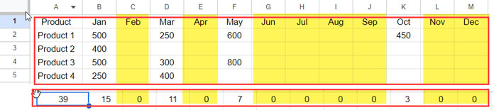
TRIM(QUERY('Test Data'!A2:M,,9^9))The LEN function converts the above result to 0 in blank columns and the count of characters in other columns.
LEN(TRIM(QUERY('Test Data'!A2:M,,9^9)))Note: If you test the formula LEN(TRIM(QUERY('Test Data'!A2:M,,9^9))) in a cell, it won’t work as expected because the QUERY function returns a range of values, and the TRIM and LEN functions can only operate on a single value. To use the formula correctly, you must use it with the ARRAYFORMULA function.
However, you can omit the ARRAYFORMULA function within the FILTER function, because the FILTER function can operate on ranges of values.
The FILTER function removes the columns if the values in the condition1 are equal to 0.
How to Remove Empty Columns and Rows in Google Sheets
Here is an additional tip.
We have seen how to filter out blank columns in Google Sheets. Now, what about filtering out blank rows and columns?
This is actually quite simple. In another tutorial, I explained how to filter out blank rows in Google Sheets. It’s titled Filter Out If the Entire Row Is Blank in Google Sheets.
We can combine both of these formulas, and it’s very simple.
In that tutorial, you can see the following formula to filter out blank rows in the range A1:G (the range is different there):
=FILTER(A1:G,LEN(TRIM(TRANSPOSE(QUERY(TRANSPOSE(A1:G),,9^9)))))To remove empty columns in the same range, we can use the following formula, which you have already seen above:
=FILTER(A1:G,LEN(TRIM(QUERY(A2:G,,9^9))))How do we combine them?
You need to replace A1:G, which appears twice in the formula that filters out blank rows, with the formula that filters out blank columns. Here is the combined formula:
=FILTER(FILTER(A1:G,LEN(TRIM(QUERY(A2:G,,9^9)))),LEN(TRIM(TRANSPOSE(QUERY(TRANSPOSE(FILTER(A1:G,LEN(TRIM(QUERY(A2:G,,9^9))))),,9^9)))))How Do We Simplify It?
Wait! I don’t recommend repeating the formula as above in an expression. That will reduce the performance. A better way to do this is to name the formula that filters out blank columns and use that name.
To name using the LET function, you can use the following syntax:
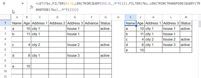
=LET(name, expression, formula)I am using the name fbc. So the formula will be:
=LET(fbc,FILTER(A1:G,LEN(TRIM(QUERY(A2:G,,9^9)))),FILTER(fbc,LEN(TRIM(TRANSPOSE(QUERY(TRANSPOSE(fbc),,9^9))))))Where:
- the
nameargument isfbc. - the
expressionargument is the formula that filters out blank columns. - the
formulaargument is the formula that filters out blank rows where the range is replaced by the namefbc, twice.
So, this way you can filter out blank rows and columns in Google Sheets using the LET function.


Hi,
Is there a way to return the same results without the first row? I need the same range, but only the data in A2:M. I’m not sure how to change it.
Hi Bryan,
I’ve completely rewritten this tutorial to include new, simple formulas. Please review them.
Hi Prashanth,
I need help regarding mixed data.
I have a Google spreadsheet with text, dates, numbers, URL columns, and a column with email IDs.
I want to filter data based on criteria, say email ID.
I tried the formula you showed but did not get the expected results.
Text and email id columns are blank, and there is also a URL column not showing as expected.
Hi, Mohammed Ahmed,
If you have a table containing mixed data, Query won’t work correctly. There may be missing info in columns in the output.
But the definition of mixed data is not a table with date, text, or number columns. But a column, e.g.:- D1:D, contains mixed-type data.
In that case, you may use the FILTER function. If you are so particular to use Query, select the mixed data type column(s) in the source table and apply Format > Number > Plain Text.
Hello Prashanth! It took me a day, but I finally got this to work on my data. It helped a lot!
Now I would like to add a dynamic total row at the end of the data that sums all the columns.
Is there any way that you might have a little bit of time to look into if that would be possible?
Appreciate your website. It has helped me so much!!! Thank you!
Hi, Noelle,
To learn how to add a total row at the bottom and a total column at the right-hand side of a table, you can follow the below tutorial.
How to Use QUERY Function Similar to Pivot Table in Google Sheets.
Anyway, feel free to share your Sheet (a sample sheet preferred) via comment. I won’t publish it.
Hi. Thanks for your hard work. I have been playing around with this for the better part of a day and have two remaining issues.
It seems to always bring in column A even if all cells are blank. I can’t figure how to not bring in that column.
It still doesn’t seem to be able to handle text data. If I use the sample data sheet and replace the numbers with the text they are picked up as non-null cells but display as blanks.
I have been able to adapt starting to look for the blanks beginning in row 4, but the above two problems are still stumping me.
Thanks
Don
Hi, D Freeland,
Thanks for reaching out to me for the help. Here are my clarifications/workarounds to your two issues with the formula.
1. It still seems unable to handle text data.
Ans:
The formula seems to work if all the columns except the first column are either text strings or numbers.
If some columns contain text and some other columns numbers, then the said issue happens.
It is because I am transferring the data at one point that makes in Query mixed data issue.
The solution is not modifying the formula. Instead, select
'Test Data'!A2:Zand go to the menu Format and apply Number>Plain Text.It solves the problem. In case you want to use the output column in any calculations, then use the VALUE function.
Eg:
=sum('Formula Output'!B2:B)It should be used as
=ArrayFormula(sum(value('Formula Output'!B2:B)))2. It seems always bringing column A values, even if all cells are blank.
Ans:
It can be easily solved using the below logical test in front of the formula.
=if(counta('Test Data'!A2:Z)=0,,formula_here)Hi! I found your resolution very interesting. Been trying to use it for an hour now but it doesn’t work for me.
I copied your test sheet. Then copied data from there to my doc – seems that it only works, when you put the formula to A1 and when the data begins in some other sheet in A1.
I need to have that output somewhere else – then I get “formula parse error” 🙁
I would like to help you. If possible, please share a sheet that contains some mockup data.
I was wondering if you could help me solve this problem.
Here is the Sheet: — URL removed —
It’s counting a blank cell when it shouldn’t. I added ‘is not null’ to both sides of the QUERY formula, but it still.
Thanks for your help!
It was nice to discuss the issue with you on the sheet. You were using the correct formula.
Cheers!
Hi,
Wonderful tutorial and well explained. Let me ask one question.
I have data for a cross country meet. The columns are Year, Name, Grade, and then like 15 Meets.
I enter their time per person in rows. So every year we run different meets.. so in 2020 we only ran 8 meets, but obviously, that means there are 7 “empty” columns.
What I would like to do is put a year drop down and then use your formula to filter the year and then run the query. Any guidance?
Hi, Brian,
I think I can set it for you. Can you share a demo sheet link/URL in your reply (it won’t be published)?
I am using this formula which works fine as long as there is more than one variable.
If there is only one it will bring over the header but not the info below, if I change the last offset in the formula from 1 to 0 it brings over the counting row and displays the info which is working, I just can’t get it to do the info and the header if there is only 1 variable
=ArrayFormula(Query(transpose(Query(TRANSPOSE({Query({A1:G1;Query({if(A2:G"",1,0)},"Select "&JOIN(",","Sum(Col"&column(A1:G1)&")"))},"Offset 1",1);A2:G}),"Select * Where Col20")),"Select * Offset 1",0))Hi, Chris,
Thanks for reporting the problem. Upon testing, I could find an issue with my formula. My formula was working well with only the columns that contain numeric values (dates or numbers).
I have updated my formula to consider text columns too. For example, now column D can contain numbers and column E can contain texts.
But never use the formula if a column contain both numbers and texts (mixed data type). Query won’t work well in that case.
I put that into my live sheet and it worked great! Thanks for the help!