Using QUERY Function Similar to a Pivot Table in Google Sheets

You can use the QUERY function to achieve similar results as a Pivot Table in Google Sheets. However, it offers more flexibility and control with its advanced filtering and data manipulation capabilities.

The QUERY function has a PIVOT clause that helps transform distinct values in columns into new columns. While it doesn’t have a built-in feature for total rows and columns like traditional Pivot Tables, we can achieve this using clever methods.

In this tutorial, we’ll create a Pivot Table using the Insert menu (I’ll just give a brief explanation as you may already be familiar with it), and a QUERY function Pivot Table (step by step).

Sample Data:

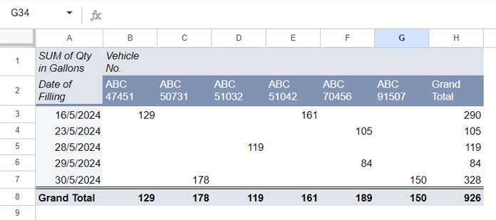
The following sample data in the range A1:C8 consists of diesel consumption of a few heavy vehicles (trucks). Let’s summarize it.

Date of Filling	Vehicle No.	Qty in Gallons
16/5/2024	ABC 51042	161
16/5/2024	ABC 47451	129
23/5/2024	ABC 70456	105
28/5/2024	ABC 51032	119
29/5/2024	ABC 70456	84
30/5/2024	ABC 50731	178
30/5/2024	ABC 91507	150

Creating a Pivot Table (Insert Menu) in Google Sheets

We will start by creating a Pivot Table using the built-in tool first, and then we’ll use the QUERY function to return a similar Pivot Table.

Select the data in A1:C8.
Click Insert > Pivot Table.
Click Create on the dialog box that appears.
In the sidebar Pivot Table editor panel, drag and drop the fields ‘Date of Filling’ under “Rows”, ‘Vehicle No.’ under “Columns”, and ‘Qty in Gallons’ under “Values”.

Your Pivot Table is ready. It’s just that simple.

An Example of a Drag-and-Drop Pivot Table in Google Sheets

Now, how do we create a similar Pivot Table using the QUERY function? Let’s find out.

Using QUERY Function Similar to Pivot Table in Google Sheets

We need to first understand which column to pivot.

Since we are following the above Pivot Table, we should pivot the field that was added to the “Columns” section in the Pivot Table settings.

If you scroll up and go through the steps, you can see that it’s the “Vehicle No.” field.

So, when we create a Pivot Table using the QUERY function, we should use the same column (field) in the PIVOT clause.

Here is the QUERY formula that uses the PIVOT clause to transform distinct values in the ‘Vehicle No.’ column into new columns:

Formula:

=QUERY(A1:C, "SELECT A, SUM(C) WHERE A IS NOT NULL GROUP BY A PIVOT B", 1)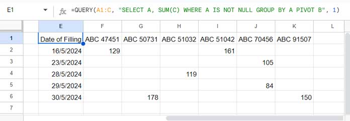

Query Pivot without a Total Row and Column

Formula Breakdown

This follows the syntax QUERY(data, query, [headers]) where:

data: A1:C (the source data range)
query: "SELECT A, SUM(C) WHERE A IS NOT NULL GROUP BY A PIVOT B" (the query to be performed)
headers: 1 (number of header rows in the source data)

Let’s break down the query string so that you can easily understand the formula:

SELECT A, SUM(C): The SELECT clause selects column A (Date of Filling) and the sum of column C (Qty in Gallons).
WHERE A IS NOT NULL: The WHERE clause filters out rows where column A (Date of Filling) is null. This omits blank rows in the source data.
GROUP BY A: This clause groups the results by the fuel filling dates in column A.
PIVOT B: This creates a Pivot Table by transforming distinct vehicle numbers in column B into new columns.

QUERY Formula That Returns Results Similar to a Pivot Table

The above QUERY formula generates a Pivot Table report similar to the one we created using the built-in tool in Google Sheets. However, it lacks the total row at the bottom and the total column on the right.

To add the total row and column, you can use the following formula. In it, you just replace query_formula with your QUERY pivot formula. A detailed explanation follows after this formula.

=ArrayFormula(LET(
   qry, 
      query_formula, 
   tab, 
      HSTACK("Total", DSUM(qry, SEQUENCE(1, COLUMNS(qry)-1, 2), IFNA(VSTACK(CHOOSEROWS(qry, 1), )))), 
   qryB, 
      VSTACK(qry, tab), 
   tar, 
      HSTACK("Total", DSUM(TRANSPOSE(qryB), SEQUENCE(1, COLUMNS(TRANSPOSE(qryB))-1, 2), IFNA(VSTACK(CHOOSEROWS(TRANSPOSE(qryB), 1), )))), 
   HSTACK(qryB, TRANSPOSE(tar))
))

Adding a Total Row and Column to the QUERY Function Pivot Table (Formula Explanation)

Here is the most interesting part of the tutorial.

The pivoted QUERY result, as shown in the image above, lacks a total row at the bottom and a column to the right.

There are mainly three approaches to adding a total row or column to a QUERY Pivot:

Using the QUERY function itself (using two more QUERY formulas, one for the total row and another for the total column)
BYCOL for the total row at the bottom and BYROW for the total column at the right
DSUM (one for the total row and one for the column).

Choosing the Best Option

QUERY will be all right, but it won’t depend on the primary result. Instead, it will use the source data to generate totals, which may occasionally lead to discrepancies in totals compared to the main QUERY Pivot.

BYCOL and BYROW are lambda helper functions. You may face issues with the header row and category column as they won’t recognize them by default, resulting in totals for those rows and columns.

DSUM is the perfect option. It’s a database function that can recognize the header row and return each column’s total at the bottom. For the total column at the right, we will transpose the data and perform a column total.

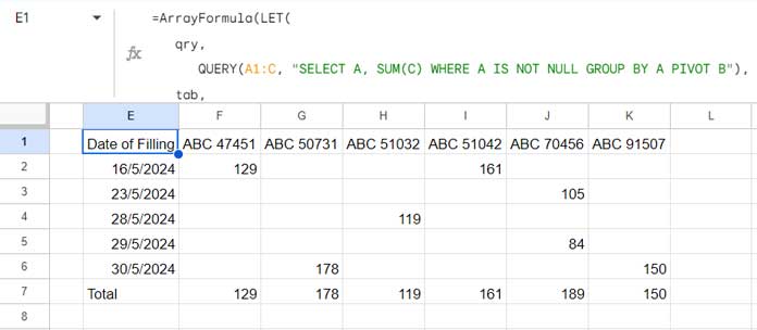
Adding a Total Row at the Bottom of the Report

Adding a Total Row to the Query Pivot Table

Generic Formula:

=ARRAYFORMULA(HSTACK("Total", DSUM(qry, SEQUENCE(1, COLUMNS(qry)-1, 2), IFNA(VSTACK(CHOOSEROWS(qry, 1), )))))

In this, you should replace wherever ‘qry’ appears with your QUERY formula, which will return the total row to add at the bottom of your QUERY Pivot Table report.

The formula adheres to the DSUM syntax DSUM(database, field, criteria) where:

database: qry – the QUERY result
field: SEQUENCE(1, COLUMNS(qry)-1, 2) – all columns in the QUERY result starting from the second column
criteria: IFNA(VSTACK(CHOOSEROWS(qry, 1), )) – the header row of the QUERY result and a blank row at the bottom, which represents no filter to apply
The HSTACK function adds the text “Total”.

Improving Performance:

Using the QUERY formula multiple times in DSUM can affect performance because of the repeated calculation. We can avoid that using the LET function.

Syntax:

LET(name1, value_expression1, [name2, …], [value_expression2, …], formula_expression)

We will assign the name ‘qry’ to the QUERY formula that returns the Pivot Table and ‘tab’ to the DSUM formula that returns the total row.

Finally, we will vertically append the DSUM total row to the QUERY result in the formula expression part.

=ArrayFormula(LET(
   qry, 
      QUERY(A1:C, "SELECT A, SUM(C) WHERE A IS NOT NULL GROUP BY A PIVOT B"), 
   tab, 
      HSTACK("Total", DSUM(qry, SEQUENCE(1, COLUMNS(qry)-1, 2), IFNA(VSTACK(CHOOSEROWS(qry, 1), )))), 
   VSTACK(qry, tab)
))

This is the proper way to add a total row at the bottom of the QUERY Pivot Table in Google Sheets.

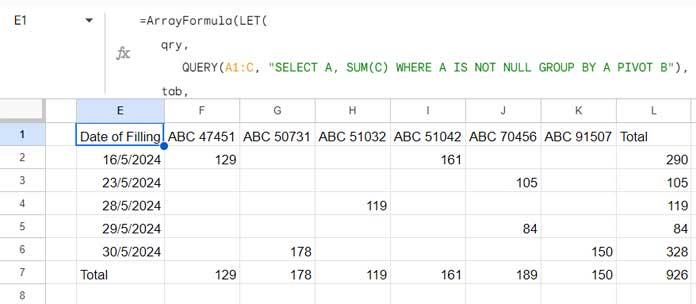
Query Function Similar to Pivot Table (After Adding a Total Row and Column)

Adding a Total Column to the Right of the Report

Here we will start with the final formula, followed by the formula explanation.

=ArrayFormula(LET(
   qry, 
      QUERY(C1:E, "SELECT C, SUM(E) WHERE C IS NOT NULL GROUP BY C PIVOT D"), 
   tab, 
      HSTACK("Total", DSUM(qry, SEQUENCE(1, COLUMNS(qry)-1, 2), IFNA(VSTACK(CHOOSEROWS(qry, 1), )))), 
   qryB, 
      VSTACK(qry, tab), 
   tar, 
      HSTACK("Total", DSUM(TRANSPOSE(qryB), SEQUENCE(1, COLUMNS(TRANSPOSE(qryB))-1, 2), IFNA(VSTACK(CHOOSEROWS(TRANSPOSE(qryB), 1), )))), 
   HSTACK(qryB, TRANSPOSE(tar))
))

We have already seen the first part where we added the total row to the Pivot Table report. Here is the rest of the explanation.

We assigned the name ‘qryB’ to the Pivot Table with the total row, i.e., VSTACK(qry, tab), and the name ‘tar’ to the new DSUM formula. Since DSUM only sums columns by default, we transposed ‘qryB’, which is the database.

Finally, the formula vertically appends the ‘qryB’ result with the transposed ‘tar’ result.

This way, we can add a total column to the right of the Pivot Table report.

Resources

Here are some related resources regarding the QUERY function’s PIVOT clause in Google Sheets.

22 COMMENTS

Neil Parris March 2, 2022 At 9:33 pm

Can you explain how to shift the grand total over when you have more than one grouping?

Say I add a location field next to the date. How do I shift the grand total numbers over to line up with the columns?

Thank you so much!

- Prashanth March 4, 2022 At 10:04 am
  
  Hi, Neil Parris,
  
  It depends on your data.
  
  You may, please, try to share a sample sheet (URL) below.
  
- Prashanth March 6, 2022 At 4:16 pm
  
  Hi, Neil Parris,
  
  Thanks for the Sheet. Inserted my formula there.
  
Guillaume January 8, 2022 At 3:49 am

How, in your example, can I sort the rows by desc the total number of vehicles?

That’s the power of pivot tables. I’m not sure it can be easily replicated via the query function.

Weston B December 29, 2021 At 3:25 am

This is amazing.

Is there anything simple that can be added to the below formula to make sure the blank cells show as “0” instead of being blank?

=QUERY(A2:C16,"SELECT C,SUM(B) GROUP BY C PIVOT A")

- Prashanth December 29, 2021 At 12:49 pm
  
  Hi, Weston B,
  
  I have seen your second question under my related tutorial. I’ll reply there.
  
  Related: Replace Blank Cells with 0 in Query Pivot in Google Sheets.
  
Ron Turnbull September 23, 2021 At 9:15 am

It took me forever to figure out why you transposed the first array.

I suppose only to make sure that the heading “vehicle number” appears at the top right; otherwise, you would get “Date of Filling.”

Still, not sure why the column label appears and not the row.

- Prashanth September 25, 2021 At 11:36 am
  
  Hi, Ron Turnbull,
  
  I assume understanding the Pivot clause may clear your doubts.
  
  This may help – What is the Correct Clause Order in Google Sheets Query?
  
  As a side note, we can avoid using Transpose in the step#1 formula as below.
  
  =QUERY(A2:C16,"SELECT A,SUM(B) GROUP BY A PIVOT C")
  
Silas Das Gupta February 16, 2021 At 9:18 pm

It is working very nicely. Thanks.

Justin August 19, 2020 At 6:49 am

Thank you for the great example.

However, I wonder if there is any advantage using Query function to pivot data comparing to making a pivot table.

- Prashanth August 19, 2020 At 10:21 pm
  
  Hi, Justin,
  
  There are a quite few. Here are two of them.
  
  We can import data using Query Importrange and pivot the data straightaway. All this we can do with a single formula.
  
  The pivot output (the formula itself) can be used as the “range” in Vlookup.
  
  In addition to this, we can take benefit of the Query complex comparison operators to fine-tune the data that we pivot.
  
shoaib June 27, 2020 At 12:49 am

Hi, Thank you for explaining this nicely in the example.

I am new to the Query function. However, from the example I understood and applied and created a report then I compared it with a pivot report just to match the figures.

There were 75 records. The values of 73 records fully matched the Query result and pivot report. However, for 2 records the Query result is different than the Pivot result. I don’t know why query function displaying the wrong result for two records. Here is a formula

=transpose(query($AB$4:$BI,"select AZ, sum(BI) where (BI > 0) group by AZ pivot AD"))

Can you look at the formula? Maybe something needs to be added here.

- Prashanth June 27, 2020 At 9:51 am
  
  Hi, Shoaib,
  
  I don’t find any issue in your formula. I would like to help you if you can share your file in viewable mode.
  
  - shoaib June 27, 2020 At 1:32 pm
    
    How to share with you in viewable mode here?
    
    - Prashanth June 27, 2020 At 2:06 pm
      
      Click the “Share” button which is in Green color on your sheet. Then copy the link and share it in the reply below. Don’t worry! I won’t publish the link.
      
Mukesh June 15, 2019 At 5:55 pm

Is there a way to sort the pivot column (row in the output).

- Prashanth June 16, 2019 At 10:11 am
  
  Hi, Mukesh,
  
  Sorting is possible with the ORDER BY clause in Query. I didn’t understand exactly your requirement.
  
  You can make an example Sheet, pivot the data and show me which column, row you want to sort.
  
  Best,
  
  - Adrax January 11, 2020 At 4:35 pm
    
    Hi, Prashanth,
    
    Having the same difficulty sorting the pivot column as well. How do I go about it to show you the sheet?
    
    - Prashanth January 11, 2020 At 10:25 pm
      
      You can use the comment form to share the link with me (EDIT or VIEW access).
      
Mayank Goel May 4, 2019 At 6:26 am

First of all the above explanation was really helpful.

The only question I have is what if I used the order by clause to order the rows or columns in a particular ascending or descending order, in that case, my grand total will not match and I couldn’t find a way to sort the grand total based on the same field as used in row and column.

- Prashanth May 4, 2019 At 11:22 am
  
  Hi, Mayank,
  
  I have added a new tab to my shared sheet labeled as “SORTing Grand Total”
  
  In that, I have modified the column C (vehicle numbers) from number to text. So that I can better experiment with sorting.
  
  Suppose I have sorted the vehicle number by descending order. The formula would be like this.
  
  See cell E3.
  
  =TRANSPOSE(QUERY(A2:C16,"SELECT C,SUM(B) GROUP BY C PIVOT A ORDER BY C DESC"))
  
  In the bottom grand total you must include the same sorting order.
  
  See cell E12.
  
  =transpose(QUERY(QUERY(A2:C16,"SELECT C,SUM(B) GROUP BY C ORDER BY C DESC LABEL SUM(B) 'GRAND TOTAL'"),"Select Col2"))
  
  Other two formulas (grand total on the right side and right side bottom) will remain the same.
  
  Best,
  
Bahadur January 15, 2018 At 4:26 pm

Hi
How to sort the output by the grans Total