Google Sheets IMPORTRANGE Function: Complete Guide with Examples

You can use the IMPORTRANGE function in Google Sheets to import data from one spreadsheet file into another. It can import ranges, named ranges, or table references from another spreadsheet.

It is one of the most useful functions when working with multiple files, shared reports, dashboards, or centralized data systems.

Please note that IMPORTRANGE works between Google Sheets files. It does not directly work with Excel files unless they are converted to Google Sheets format.

While you can also use IMPORTRANGE within the same spreadsheet file, I generally don’t recommend it. In most cases, functions like QUERY, FILTER, or ARRAYFORMULA are more efficient. I mainly use same-file IMPORTRANGE only for testing formulas.

In this tutorial, we will explore both basic and advanced uses of the Google Sheets IMPORTRANGE function.

Table of Contents

What Is IMPORTRANGE in Google Sheets?

The IMPORTRANGE function pulls data from one Google Sheets file into another.

Common uses include:

Creating dashboards from source files
Sharing reports without exposing raw data
Combining team spreadsheets
Pulling data from separate workbooks automatically

IMPORTRANGE Function Syntax

IMPORTRANGE(spreadsheet_url, range_string)

Arguments

spreadsheet_url
The URL of the source spreadsheet from which data will be imported.

You can either:

Hardcode the URL inside double quotes
Use a cell reference containing the URL

range_string
The range to import.

Examples:

"Sheet1!B1:N100"
"Class Data!A:F"
"B1:N100"

If you omit the sheet name, Google Sheets imports from the first sheet in the source file.

You can also use named ranges or structured table references, such as:

"SalesData"
"Table1[#ALL]"

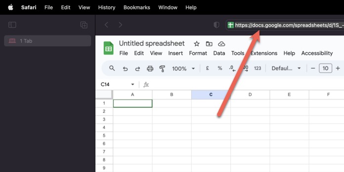
How to Copy the Source Spreadsheet URL

To use the IMPORTRANGE function:

Open the source spreadsheet.
Click in the browser address bar.
Copy the URL using:

Ctrl + C (Windows)
⌘ + C (Mac)

You can now use that URL inside the formula.

Google Sheets source file URL highlighted in Safari browser address bar

How to Use IMPORTRANGE in Google Sheets

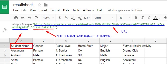
Assume there are two files:

MasterFile (source)
ResultSheet (destination)

The data in MasterFile is in:

Class Data!A:F

Go to the destination file and enter:

=IMPORTRANGE("paste-source-url-here", "Class Data!A:F")

This imports columns A to F from the source file.

IMPORTRANGE formula in Google Sheets showing highlighted URL and range_string with imported results

Fixing #REF! Errors in the IMPORTRANGE Function

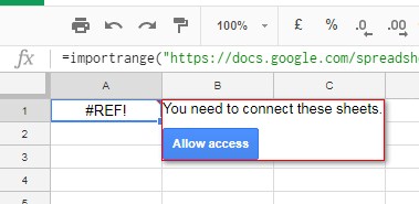
First-Time Access Error

When connecting two spreadsheets for the first time, Google Sheets may return a #REF! error.

Hover over the error and click Allow access.

Once approved, the data will load normally.

Allow Access option for #REF! error in Google Sheets IMPORTRANGE function

If clicking Allow access does not solve the issue:

Check the URL

Make sure the spreadsheet URL is correct.

If you are not the owner, ask the owner to share the source file with you.

Check range_string

Verify:

Sheet name spelling
Range reference
Named range name

Still Not Working?

Try:

Reloading the spreadsheet
Clearing browser cache/cookies
Re-entering the formula

Use Cell References Instead of Hardcoding

Instead of placing everything inside the formula:

A1 = spreadsheet URL
A2 = Class Data!A:F

Use:

=IMPORTRANGE(A1, A2)

This method makes formulas easier to edit later.

Can I Use Named Ranges as range_string?

Yes.

If the source file contains a named range called SalesData, use:

=IMPORTRANGE("source-url", "SalesData")

Named ranges are useful when the source range may grow or shift.

Related tutorial: IMPORTRANGE Named Ranges in Google Sheets

Can I Use Table References as range_string?

Yes. Google Sheets now supports structured table references.

Suppose the source file contains a table named Table1.

Examples:

=IMPORTRANGE("source-url", "Table1[#ALL]")
=IMPORTRANGE("source-url", "Table1")
=IMPORTRANGE("source-url", "Table1[[#ALL],[Status]]")
=IMPORTRANGE("source-url", "Table1[Status]")
=IMPORTRANGE("source-url", "Table1[[#ALL],[Item]:[Amount]]")
=IMPORTRANGE("source-url", "Table1[[Item]:[Amount]]")

Meaning

Table1[#ALL] → Entire table including headers
Table1 → Table body only
Table1[[#ALL],[Status]] → Only the Status column with header
Table1[Status] → Only the Status column without header
Table1[[#ALL],[Item]:[Amount]] → Consecutive columns from Item to Amount, including headers
Table1[[Item]:[Amount]] → Consecutive columns from Item to Amount, without headers

If you need non-adjacent columns or more advanced filtering, import the table first and then use CHOOSECOLS, FILTER or QUERY.

Performance Tips for IMPORTRANGE

If your file becomes slow, try these tips.

Use Fewer IMPORTRANGE Formulas

Too many separate imports can slow recalculation, and when several files are linked using IMPORTRANGE, updates may take longer.

Use Smaller Ranges

Instead of:

A:Z

Use:

A1:Z1000

Import Once, Analyze Locally

Import data to one helper tab, then use QUERY, FILTER, VLOOKUP, or XLOOKUP on that imported data.

IMPORTRANGE Resources

We have many tutorials covering advanced uses of the IMPORTRANGE function.

Lookups

QUERY and Conditions

Dynamic References

Summing and Combining

Filtering

Troubleshooting

Frequently Asked Questions

Can I use IMPORTRANGE with Excel files?

Not directly. Convert the file to Google Sheets first.

Can I use IMPORTRANGE inside the same file?

Yes, but QUERY, FILTER, or ARRAYFORMULA are usually better choices.

Why is IMPORTRANGE slow?

Usually because of multiple imports, large ranges, or chained formulas.

Can I combine QUERY with IMPORTRANGE?

Yes. QUERY with IMPORTRANGE is one of the most popular combinations for filtering imported data.

Conclusion

The Google Sheets IMPORTRANGE function is one of the easiest ways to connect spreadsheets and automate reporting.

Start with a simple import, then combine it with QUERY, FILTER, VLOOKUP, or XLOOKUP for advanced workflows.

If you frequently work with multiple files, mastering IMPORTRANGE will save you a lot of time.

24 COMMENTS

Ameya Raje February 28, 2020 At 4:20 pm

Hi,

I have a Google Sheet from where I import the columns using Query and Importrange functionality into another Google Sheet.

I mark some comments in the new Google Sheet against the rows that are imported. But when the new rows get amended (using Query and Importrange) the comments marked for these also are shuffled. Any way I can lock those comments or those rows?

- Prashanth February 29, 2020 At 8:54 am
  
  Hi, Ameya Raje,
  
  That’s only possible with a common ID column as detailed in this guide – Align Imported Data with Manually Entered Data in Google Sheets.
  
andrew January 23, 2020 At 3:41 am

Hi,

Is there a way that I could stop an importrange from updating? or someway to only reload the data with a button press or a checkbox tic? I have a file with a schedule that I am mirroring to another workbook and I don’t want others to see the changes before they’re ready.

- Prashanth January 23, 2020 At 9:08 am
  
  Hi, Andrew,
  
  We can control the import with a tickbox inserting in the source file. I’ll test it myself and update you very soon.
  
- Prashanth January 23, 2020 At 5:05 pm
  
  How to Control Reloading of Importrange from the Source File in Google Sheets
  
Lili October 10, 2019 At 10:49 pm

Hi!

Is there a way to import data from one sheet to another sheet only when the checkbox is marked?

If so, how do I do it?

Thanks for all your help, these tutorials are great!

- Prashanth October 11, 2019 At 11:06 am
  
  Hi, Lili,
  
  Checkbox marked on which Sheet. Source sheet or the Sheet containing the Importrange formula?
  
  Please clarify.
  
  Best,
  
William May 27, 2019 At 7:28 pm

Hello,

I have multiple spreadsheets that are tabbed “Wk1” – “Wk52”, and I’m using importrange within the sheets.

However, I am trying to figure out a way to make the range_string part of the formula grab a cell within the sheet that I have the formula in so that it knows what tab I want data from.

Not sure if this is possible?

So if I have a cell D3 with the value 21 in my current sheet (because I want data from Wk21), how could I correctly input the formula? I’m trying similar to this so far, but with no luck –

=importrange("url","Wk"D3"!A2")

- Prashanth May 28, 2019 At 8:37 am
  
  Hi, William,
  
  Your formula to get dynamic tab names in Importrange must be as follows.
  
  =importrange("url","Wk"&D3&"!A2")
  
  I think you have missed my tutorial Dynamic Tab Names in Importrange.
  
  There you can find a similar solution using named ranges.
  
  Best,
  
Desmond LEE May 5, 2019 At 6:29 am

Hi There,

Importrange shows only the header in the Query. When I delete the query and manually type value everything is pulled to another sheet.

This is the query.

=QUERY('WO Start Rev 03 -1'!A:J, "SELECT A,C,I,F WHERE C MATCHES '"&JOIN("|",C:C)&"'")

This is the importrange formula.

=IF(ISERROR(ImportRange("URL","QA")), IF(ISERROR(ImportRange("URL","QAB")),ImportRange("URL","QAC"), ImportRange("URL","WO!Q:q")),ImportRange("URL","WO!q:Q"))

- Prashanth May 5, 2019 At 9:19 am
  
  Hi, Desmond LEE,
  
  The Query formula must be in this pattern. See the TEXTJOIN function used instead of JOIN.
  
  =QUERY(A1:D,"SELECT A,B,C,D WHERE C MATCHES "&"'"&textjoin("|",true,G1:G)&"'")
  
  When you replace A1:D (data) with the above importrange, you must change the column identifiers in SELECT clause and as well as in WHERE clause.
  
  For example, you must use the formula as below.
  
  =QUERY(importrange formula here,"SELECT Col1,Col2,Col3,Col4 WHERE Col3 MATCHES "&"'"&textjoin("|",true,G1:G)&"'")
  
  I have updated my post to include additional resources at the bottom. Please go thru’ that too for some awesome importrange related tips.
  
  Best,
  
Mel March 21, 2019 At 10:56 pm

Hi,

Is there a way to ensure that the font/size/color/bold/underline etc. import along with the content in the tab and ranges?

I used the importrange according to your example but it defaulted to the regular font, size etc.

Thanks!

- Prashanth March 22, 2019 At 2:01 pm
  
  Hi, Mel,
  
  If you want to import data and also keep the ‘characteristics’ of the data, you can follow the below workaround.
  
  1. Go to the Source file (File A).
  2. Click File > Make a copy. It will make a duplicate copy of the source file (Copy of File A).
  3. Delete all the contents in this ‘Copy of File A’.
  4. Import the content from ‘File A’ to ‘Copy of File A’.
  
  Best,
  
Tom January 26, 2019 At 2:36 am

I using Importrange with Vlookup and am getting the #REF! error as it is evaluating “to an out of bounds range.”
My formula is as follows (note I have substituted “key” for the actual key)

=VLOOKUP(A3&"", IMPORTRANGE("key","Duane!A2:P"),8,FALSE)

The only thing I can think of is that it is a permissions issue but I can’t get the “allow access” bubble to pop up. Is there something else I may be missing?

Thanks!

- Prashanth January 26, 2019 At 9:47 am
  
  Hi, Tom,
  
  The problem is the Importrange is not importing the data. So Vlookup has no column 8 to return value.
  
  First use importrange individually. Allow permission and then use it inside Vlookup as the range.
  
  Additionally, I have Vlookup + Importrange tutorial.
  
  How to Vlookup Importrange in Google Sheets [Formula Examples]
  
  Best,
  
maria November 9, 2018 At 2:29 pm

Hello! Thanks much for the guide. Is there a way to allow the person with whom we share the document by IMPORTRANGE to edit the sheet and both have live updates? Like in cloud? Thanks.

- Prashanth November 9, 2018 At 2:55 pm
  
  Hi, Maria,
  
  I fear I didn’t understand your question correctly. I guess you are talking about sharing Google Sheets file with edit access.
  
  You can share any Google Sheets file with Edit access. To do that look for the blue button labeled as Share on your Google Sheets. It’s on the top right-hand side of your screen.
  
  You can also share a file in just view or comment mode. You can see that options once you click on the said blue button.
  
  There is one more method in file sharing in Google Sheets but not official. It’s COPY mode.
  
  Share Google Sheet Files on Copy Mode
  
Peter Frost September 17, 2018 At 12:51 pm

Hi,

Is there a way to use IMPORTRANGE over multiple cells ?

Suyog August 29, 2018 At 11:51 am

If sheet is protected how we can use importrange function

- Prashanth August 29, 2018 At 4:48 pm
  
  Hi, Suyog,
  
  I don’t think it will affect the importrange. In my testing, the Importrange function works well with a protected sheet.
  
  Have you faced any issue? If then, what the error message says?
  
Tori August 17, 2018 At 1:45 am

Thanks for sharing, this is great! Is there a way to ‘lock’ this formula on the content you’re really looking for. For example, if I’m using the import range function on cell C5 in doc ‘123’ and the editor of doc ‘123’ adds a row to the top of doc ‘123’, it would bump the cell I need to C6. Any way I can ensure the import range function is smart enough to update my formula as things in the source sheet shift?

- Prashanth August 17, 2018 At 9:29 am
  
  Hi, Tori,
  
  Good question! I have this already addressed in an earlier tutorial. Here you go.
  
  https://infoinspired.com/google-docs/spreadsheet/freeze-cell-in-importrange-in-google-sheets/
  
  I hope it could be useful.
  
  Cheers!
  
Songthang July 19, 2018 At 12:55 pm

Hi,

I have a question. Could we draw a chart by directly using Importrange Data? Because I have many files but would like to show the chart in one specific sheet.

Thank you in advance 🙂

- Prashanth July 19, 2018 At 1:11 pm
  
  Hi, Songthang,
  
  You can create a chart from the imported data. I don’t find any issue in that.